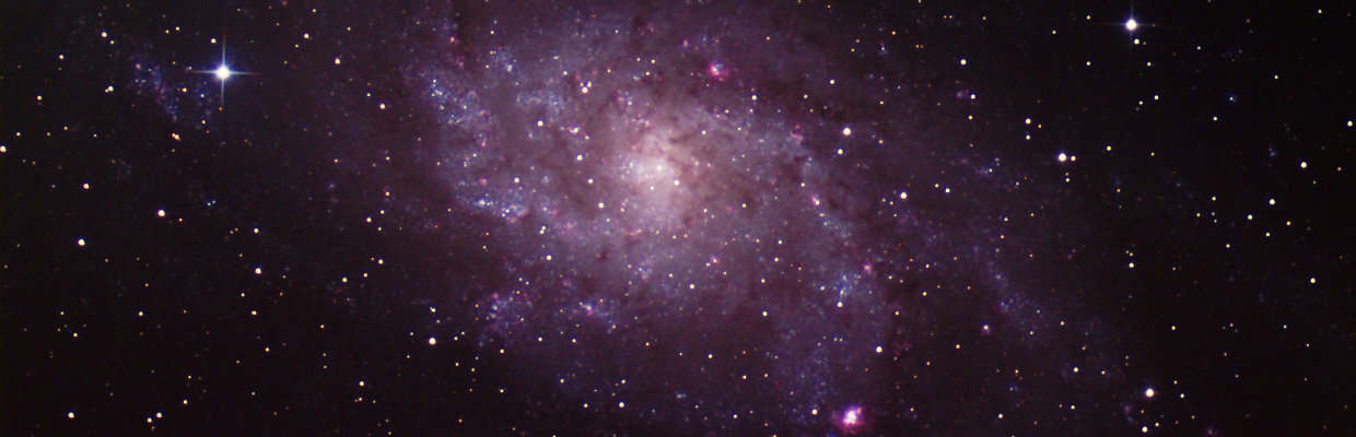

This article is about image binarization using the Otsu method. A simple C++ implementation of the Otsu thresholding algorithm based on the CImg library is shown. In Part 1 of my “Night sky image processing” series I have taken a look on anisotropic diffusion in order to reduce the image noise.
Introduction to Thresholding
The next topic I want to have a look at is thresholding. In this step the algorithm decides which pixels belong to the background and which pixels belong to a star. However, before the algorithm can decide which pixels belong to a particular star (also called clustering – see part 3) it first has to generally decide which pixels belongs to any star and which pixels belong to the background. This process is called thresholding i.e. converting a grey-scale image into a binary image. There are many different thresholding algorithms out there. All have there advantages and drawbacks. I found ImageJ very helpful to test different thresholding algorithms.
Why Otsu Thresholding for astro images
After trying different ones I found that Otsu’s method does a quite good job. After further reading I found out that this method is especially useful for images with bi-modal histograms. To my knowledge night shy images usually do not have bi-modal histograms. However, so far Otsu’s method still gave very good results with my star images. Furthermore it is relatively efficient and simple to implement. For those reasons I decided to go this way.
Introduction to Otsu Thresholding
Otsu’s algorithm tries to find the threshold so that the variance of all pixel values in the foreground and the variance of all pixel values in the background becomes minimal. The variance is a measure of the spread. The smaller the variance of for example the foreground pixel values, the closer the gray levels of the pixels and the more likely it is that they belong together. At least that’s how I understand Otsu’s method.
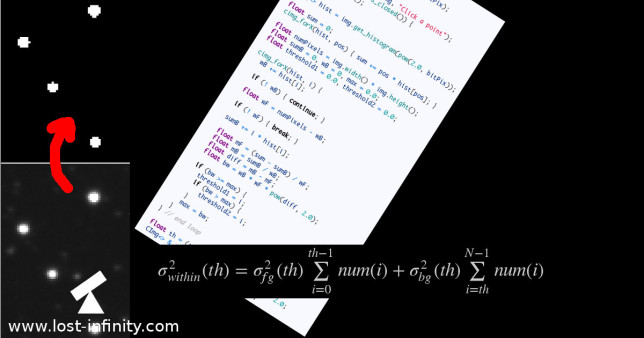
The following formula calculates a kind of “mean” variance $\sigma^2_{within}(th)$ of the foreground variance $\sigma^2_{fg}(th)$ and the background variance $\sigma^2_{bg}(th)$. In fact it is no mean but a weighted sum of both. The weights are the number of pixels in the respective group:
$$\sigma^2_{within}(th)=\sigma^2_{fg}(th) \sum\limits_{i=0}^{th-1} {num(i)} + \sigma^2_{bg}(th) \sum\limits_{i=th}^{N-1} {num(i)}$$
while $num(i)$ is the number of pixels with intensity / grey value $i$ (i.e. histogram), $th$ is a threshold value for witch the “within” variance $\sigma^2_{within}(th)$ is to be minimized, $\sigma^2_{fg}(th)$ is the variance of all the pixels in the foreground group for the given $th$, $\sigma^2_{bg}(th)$ is the variance of all the pixels in the background group for the given $th$ and $N$ is the number of grey levels (e.g. 65535 for a 16 bit image) – iterating from $0..N-1$.
As mentioned above, both variances have to be minimized for the same $th$. Now, we can minimize $\sigma^2_{within}(th)$ instead.
Finding the threshold
Finding the $th$ which minimizes $\sigma^2_{within}(th)$ is a computationally intensive task. However, thanks to Otsu, there is a quicker way to compute the best $th$. Instead of finding the $th$ that minimized $\sigma^2_{within}(th)$, one can instead calculate the “between”-variance. Then, instead of finding the $th$ that minimized $\sigma^2_{within}(th)$ one can instead try to find the $th$ that maximized the “between”-variance $\sigma^2_{between}(th)$ which is much quicker to calculate. The implementation below uses recursion formulas which are derived in detail here. In addition the following links were quite useful:
- https://en.wikipedia.org/wiki/Otsu%27s_method
- https://homepages.inf.ed.ac.uk/rbf/CVonline/LOCAL_COPIES/MORSE/threshold.pdf
Otsu Thresholding C++ Implementation
NOTE: All the source codes of this “Night sky image processing” series presented in part 1-7 are also available on github in the star_recognizer repository.
The following code is a C++ implementation of the described algorithm:
#include <iostream>
#include <algorithm>
#include <assert.h>
#include <CImg.h>
#include <CCfits/CCfits>

using namespace cimg_library;
using namespace CCfits;
using namespace std;

void readFile(CImg<float> & inImg, const string & inFilename, long * outBitPix = 0) {
  std::auto_ptr<FITS> pInfile(new FITS(inFilename, Read, true));
  PHDU & image = pInfile->pHDU();

  if (outBitPix) {
    *outBitPix = image.bitpix();
  }

  inImg.resize(image.axis(0) /*x*/, image.axis(1) /*y*/, 1/*z*/, 1 /*1 color*/);

  // NOTE: At this point we assume that there is only 1 layer.
  std::valarray<unsigned long> imgData;
  image.read(imgData);
  cimg_forXY(inImg, x, y) { inImg(x, inImg.height() - y - 1) = imgData[inImg.offset(x, y)]; }
}

int main(void) {
  CImg<float> img;
  long bitPix = 0;
  readFile(img, "test.fits", & bitPix);

  // Display initial image
  CImgDisplay imgDisp(img, "Click a point");
  while (! imgDisp.is_closed()) {
    imgDisp.wait();
  }

  CImg<> hist = img.get_histogram(pow(2.0, bitPix));

  float sum = 0;
  cimg_forX(hist, pos) { sum += pos * hist[pos]; }

  float numPixels = img.width() * img.height();
  float sumB = 0, wB = 0, max = 0.0;
  float threshold1 = 0.0, threshold2 = 0.0;

  cimg_forX(hist, i) {
    wB += hist[i];

    if (! wB) { continue; }

    float wF = numPixels - wB;

    if (! wF) { break; }

    sumB += i * hist[i];

    float mF = (sum - sumB) / wF;
    float mB = sumB / wB;
    float diff = mB - mF;
    float bw = wB * wF * pow(diff, 2.0);

    if (bw >= max) {
      threshold1 = i;
      if (bw > max) {
         threshold2 = i;
      }
      max = bw;
    }
  } // end loop

  float th = (threshold1 + threshold2) / 2.0;
  CImg<> & thImg = img.threshold(th);

  // Display result
  CImgDisplay imgDisp2(thImg, "Result");
  while (! imgDisp2.is_closed()) {
    imgDisp2.wait();
  }
  return 0;
}
The code can be compiled easily using the following command:
g++ -std=c++11 threshold_max_entropy.cpp -o threshold_max_entropy -lcfitsio -lCCfits -lX11 -lpthread
You can download the complete source here. Below is an image where the effect of Otsu’s method is shown. In Part 3 of my “Night sky image processing” series I will have a closer look on star clustering.

1 Comment