


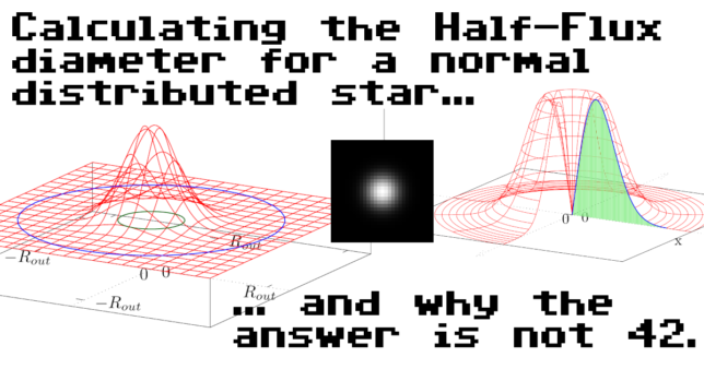
Calculating the Half Flux Diameter for a perfectly normal distributed star…
… and why the answer is not 42.
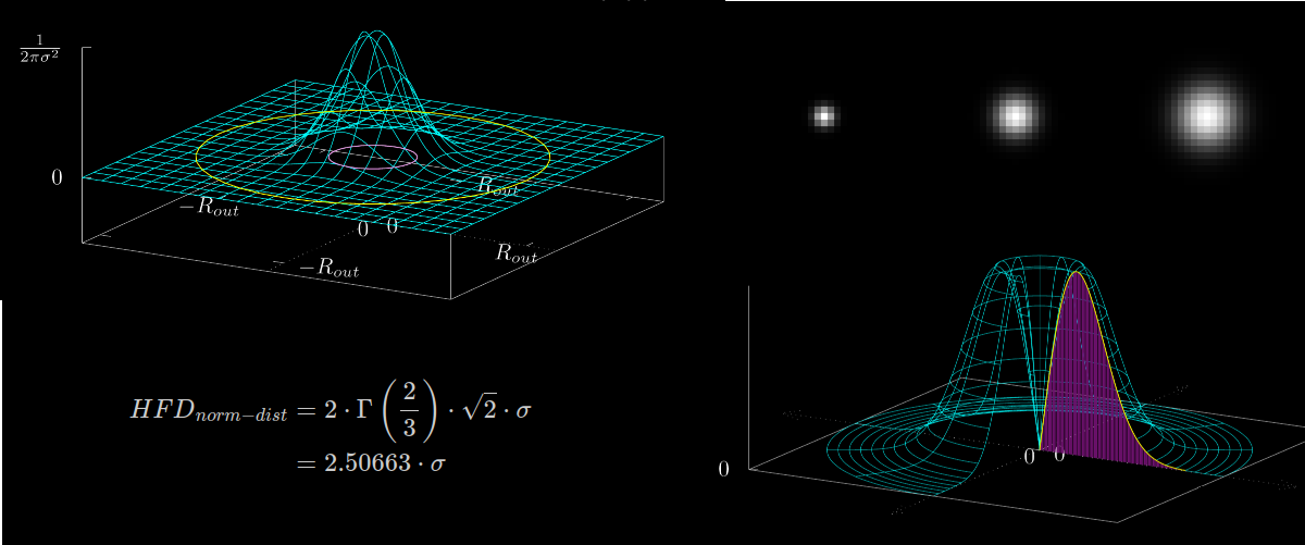
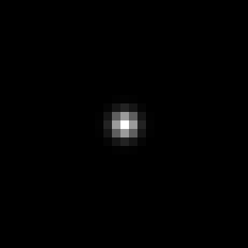
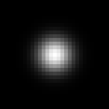
The goal of this article is to “manually” calculate the Half Flux Diameter (HFD) for a perfectly normal distributed star. Initially, I decided to add perfectly normal distributed stars with different σ values as additional unit tests to my focus finder software project. A few of those star images with σ=1, 2 and 3 are illustrated in figure 1.
Previously, I examined the Half Flux diameter (HFD) for a plain image. In that article I cover some aspects in greater detail which I am reusing in this article. If something is unclear I recommend to read this article first.

A 2D image can be represented in the 3D space where the $x$- and $y$-axis are used to express the position of the pixel and the $z$-axis to visualize the intensity (pixel value) – see figure 2 below.

Following a similar approach like for the plain image, the Half Flux Diameter (HFD) for such an image will be derived in the following sections.
Quick summary
For those who just seek for the facts – here is a quick summary:
- The Half Flux Diameter ($HFD$) for a perfectly normal distributed star is $HFD_{norm-dist} = 2 \cdot \Gamma\left(\frac{2}{3}\right) \cdot \sqrt{2} \cdot \sigma = 2.50663 \cdot \sigma$ where $\sigma$ is the variance of the distribution.
- The result does not depend on $R_{out}$ and also not on the normalization factor of the distribution.
- The expression was derived by converting the $HFD$ formula into an integral and inserting the normal distribution function as intensity (pixel value). The integral was solved by using a relation between the normal distribution and the $\Gamma$-function.
- For the volume integration the second Pappus–Guldinus theorem is used.
Recap – The Half Flux Diameter for a plain image
Before jumping right into the deviation of the Half Flux Diameter ($HFD$) for a perfectly normal distributed star, it makes sense to quickly recap the approach which was taken to deviate the $HFD$ for a plain image. If this summary is hard to understand, more details can be found in the article The Half Flux Diameter of a plain image.
The Half Flux Radius ($HFR$) is defined as
$$HFR = \frac{WDS}{PVS}=\frac{\sum\limits_{i=0}^{N-1} V_i \cdot d_i}{\sum\limits_{i=0}^{N-1} V_i}$$
For the plain image it was possible to pull the $V=V_i$ in front of the sum because all pixels had the same intensity:
$$WDS = V \cdot \sum\limits_{i=0}^{N-1} d_i $$
For one part of the sum it was then possible to rewrite the sum as an integral:
$$V \cdot \sum\limits_{i=k}^{l} d_i \simeq V\cdot \int_{0}^{R_{out}} r dr$$
In case of normal distributed pixel values the values are different, i.e. $V_i \neq V$. Instead, of pulling the $V$ in front of the sum, now the normal distribution $g(r)$ needs to be part of the integral:
$$\sum\limits_{i=k}^{l} V_i \cdot d_i \simeq \int_{0}^{R_{out}} g(r) \cdot r dr$$
In the following section the equation for the normal distribution $g(r)$ will be derived.
Deriving the normal distribution function $g(r)$
Since the normal distribution can be explicitly expressed as a formula, the image of a normal distributed star will be expressed by a function $z=f(x,y)$ in the following sections. The common bivariate normal distribution (see wikipedia) is a good starting point:
$$f(x,y)=\frac{1}{2\pi\sigma_x\sigma_y\sqrt{1-\rho^2}}\exp{\left(-\frac{1}{2(1-\rho^2)^2}\left[\left(\frac{x-\mu_x}{\sigma_x}\right)^2-2\rho\left(\frac{x-\mu_x}{\sigma_x}\right)\left(\frac{y-\mu_y}{\sigma_y}\right)+\left(\frac{y-\mu_y}{\sigma_y}\right)^2\right]\right)}$$
For the purpose of a perfectly normal distributed star this expression can be simplified a lot. First of all, the correlation between the variables $x$ and $y$ can be assumed as $0$:
$$\rho=0$$
Furthermore, the variance for $x$ and $y$ is expected to be the same (an ideal star is perfectly circular):
$$\sigma_x^2 = \sigma_y^2 = \sigma^2$$
Additionally, the mean for $x$ and $y$ is set to $0$ since the center of the star cen be assumed to be at $(0,0)$. This simplifies the equation.
$$\mu_x=\mu_y=0$$
This results in a simplified version of $f(x,y)$:
$$f(x,y)=\frac{1}{2\pi\sigma^2}\exp{\left(-\frac{1}{2}\cdot\frac{x^2+y^2}{\sigma^2}\right)}$$
Figure 3 shows $f(x,y)$ as a 3D plot (red). The blue line illustrates the function $g(x) = f(x, 0)$ which is a vertical cut through the 3D plot. This function $g(x)$ is very similar to the 1D normal distribution function – the only difference is the normalization factor which in this case is $\frac{1}{2\pi\sigma^2}$ instead of $\frac{1}{\sqrt{2\pi}\sigma}$.

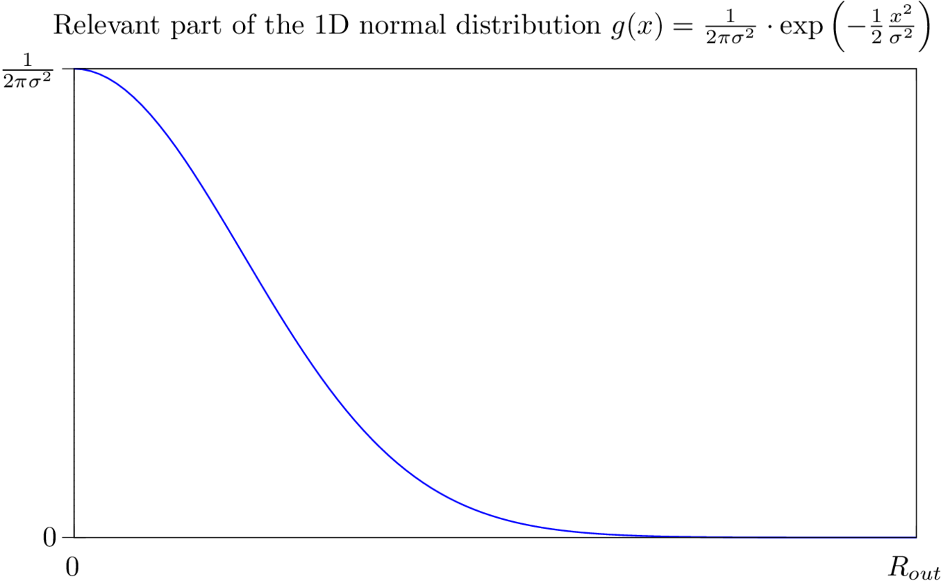
For the next step only the “right” part of $g(x)$ is relevant – i.e. $0 \leq x \leq R_{out}$. Since $g$ will later be rotated around the $z$-axis, $x$ will be from now on replaced by $r$. Setting $y=0$ in $f(x,y)$ directly results in $g(r)$:
$$g(r)=\frac{1}{2\pi\sigma^2}\exp{\left(-\frac{1}{2}\left[\frac{r}{\sigma}\right]^2\right)}, r \geq 0$$
Figure 4 illustrates $g(r)$:
Calculating the Half Flux Diameter for the normal distribution $g(r)$
$g(r)$ expresses the intensity (pixel values) depending on the distance $r$ from the star center. Therefore, $g(r)$ will replace $V_i$ in the original $HFR$ equation. As a recap $HFR$ is again written down here:
$$HFR = \frac{WDS}{PVS} = \frac{\sum\limits_{i=0}^{N-1} V_i \cdot d_i}{\sum\limits_{i=0}^{N-1} V_i}$$
The calculation will take place in two steps:
- The enumerator – the weighted distance sum ($WDS$)
- The denominator – the pixel value sum ($PVS$)
Part 1 – Calculating the Weighted Distance Sum ($WDS$)
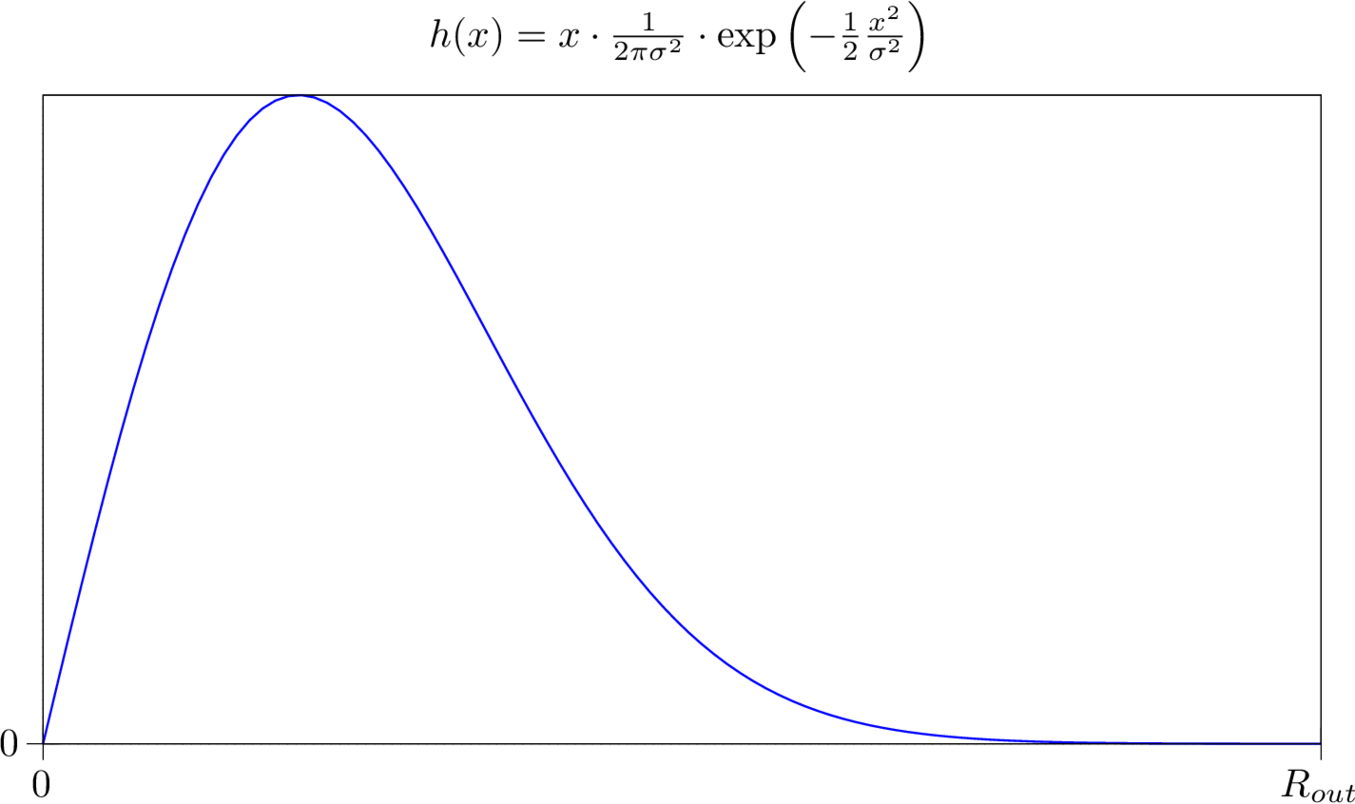
In this section the upper part of the $HFR$ equation – the weighted distance sum $WDS$ will be solved for a perfectly normal distributed star. As previously demonstrated for the plain image, the value of $WDS$ corresponds to volume under the surface which is formed when the function $h(r) = r \cdot g(r)$ is rotated around the $z$-axis.
The function $h(r)$ is given as:
$$\begin{align}
h(r) &= r \cdot g(r) \\
&= r \cdot \frac{1}{2\pi\sigma^2} \exp{\left(-\frac{1}{2}\left[\frac{r}{\sigma}\right]^2\right)} \\
\end{align}$$
A graphical representation of $h(r)$ is shown in figure 5.
In the next step the area $A_{h(r)}$ below the curve $h(r)$ is determined. One part of the sum of $WDS$ can be expressed as
$$\begin{align}
A_{h(r)}&=\sum\limits_{i=k}^{l} V_i \cdot d_i \\
&\simeq \int_{0}^{R_{out}} h(r) dr \\
&= \int_{0}^{R_{out}} r \cdot g(r) dr \\
&= \int_{0}^{R_{out}} r \cdot \frac{1}{2\pi\sigma^2}\exp{\left(-\frac{1}{2}\left[\frac{r}{\sigma}\right]^2\right)} dr \\
\end{align}$$
At this point I was stuck for a moment since I had no idea how to solve this integral analytically. However, luckily there is a way to rewrite this integral using the $\Gamma$-function:
$$\int_{0}^{\infty}x^n\cdot e^{-ax^2}dx =\frac{\Gamma\left(\frac{n+1}{2}\right)}{2a^{\frac{n+1}{2}}}$$
for $a>0, n>-1$.
The next step is to transform the integral so that it is easier to match the corresponding parameters $n$ and $a$. Furthermore, the upper limit of the integral $R_{out}$ can be replaced by $\infty$ since $h(r)$ converges against $0$.
$$\begin{align}
A_{h(r)} &= \frac{1}{2\pi\sigma^2}\cdot \int_{0}^{R_{out}} r \cdot \exp{\left(-\frac{1}{2}\left[\frac{r}{\sigma}\right]^2\right)} dr \\
&=\frac{1}{2\pi\sigma^2}\cdot \int_{0}^{\infty} r^1 \cdot \exp{\left(-\frac{1}{2\sigma^2}\cdot r^2\right)} dr
\end{align}$$
Comparing the integral against the left part of the expression above, gives
$$n=1$$
$$a=\frac{1}{2\sigma^2}$$
Putting in those values back into the right part of the expression results in
$$\begin{align}
A_{h(r)} &=\frac{1}{2\pi\sigma^2}\cdot \int_{0}^{\infty} r^1 \cdot \exp{\left(-\frac{1}{2\sigma^2}\cdot r^2\right)} dr \\
&= \frac{1}{2\pi\sigma^2}\cdot\frac{\Gamma(1)}{2a^1} \\
&= \frac{1}{2\pi\sigma^2}\cdot\frac{\Gamma(1)}{2\cdot\frac{1}{2\sigma^2}} \\
&= \frac{\Gamma(1)}{2\pi}\\
&=\frac{1}{2\pi}
\end{align}$$
That means, the area below the function $h(r)$ is equal to $\frac{1}{2\pi}$.
The next step is to calculate the volume of $h(r)$ when it is rotated around the $z$-axis (see figure 6).

One way would be to compose an infinitesimal small volume element consisting of $A_{h(r)}$ and a $d\phi$ and then integrated over $d\phi$ for $0$ to $2\pi$. However, there is another way to calculate the volume of the body – the second Pappus–Guldinus theorem:
The second theorem states that the volume V of a solid of revolution generated by rotating a plane figure F about an external axis is equal to the product of the area A of F and the distance d traveled by the geometric centroid of F.
Wikipedia / Pappus of Alexandria and Paul Guldin
So what exactly does that mean in this context? In this case it boils down to three steps:
- Calculation of the geometric centroid of $A_{h(r)}$
- Calculation of the distance $C$ the geometric centroid “travels” while rotating around the $z$-axis
- Calculation of the volume $V$ of the body according to the described rule $V=A_{h(r)} \cdot C$
In this case, since it is a rotation around the $z$-axis, the “traveled” distance of the geometric centroid is just the circumference $C$ of a circle with the radius of the $x$ component of the geometric centroid $x_c$:
$$C=2\pi x_c$$
With this the volume $V$ of the body (which corresponds to the $WDS$ term) can be calculated as
$$\begin{align}
WDS&=V\\
&=A_{h(r)}\cdot C \\
&=\frac{1}{2\pi}\cdot2\pi\cdot x_c \\
&=x_c
\end{align}$$
So what remains is the calculation of $x$-component $x_c$ of the geometric centroid of $A_{h(r)}$.
After some research I realized that the calculation of the geometric centroid of a curvilinear trapezoid is what is needed in this case (see figure 7 below).
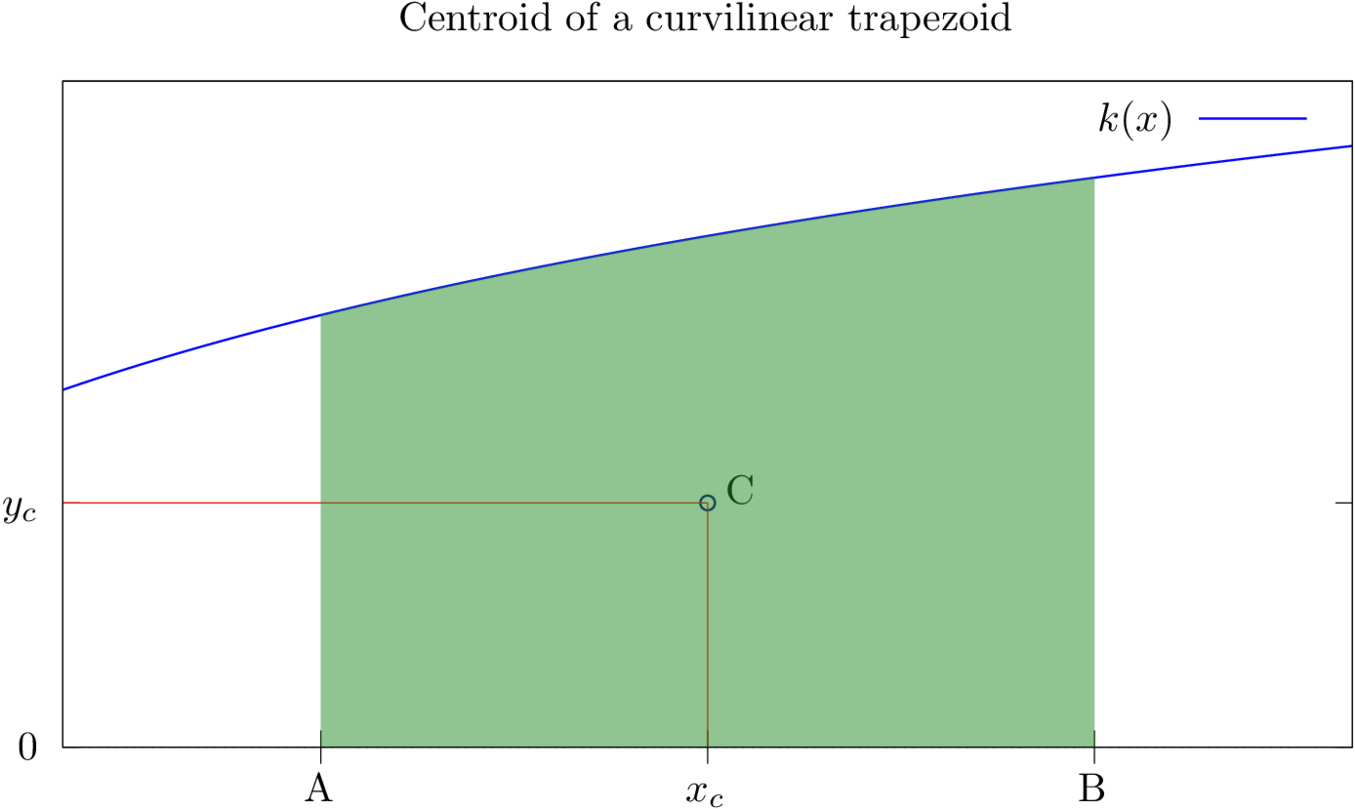
According to Wikipedia, the geometric centroid of an area which is defined by the boundaries $A$ and $B$, a curvilinear trapezoid (in this case $h(r)$ with $A=0$ and $B=\infty$) and the $x$-axis, can be calculated as
$$x_c=\frac{\int_{A}^{B}xydx}{S}$$
$$y_c=\frac{\frac{1}{2}\int_{A}^{B}y^2dx}{S}$$
where $S$ is the area of the trapezoid. In this case $S$ is already known:
$$S = A_{h(r)} = \frac{1}{2\pi}$$
As already mentioned above, in this context only $x_c$ is needed. Inserting $h(r)$ into the integral results on the following expression for $x_c$:
$$\begin{align}
x_c &= \frac{\int_{0}^{\infty}r\cdot h(r) dr}{\frac{1}{2\pi}} \\
&=2\pi\cdot \frac{1}{2\pi\sigma^2} \cdot \int_{0}^{\infty}r^2 \cdot \exp{\left(-\frac{1}{2\sigma^2}\cdot r^2\right)} dr \\
\end{align}
$$
Again the relation between the normal distribution and $\Gamma$-function comes to the rescue:
$$\int_{0}^{\infty}x^n\cdot e^{-ax^2}dx =\frac{\Gamma\left(\frac{n+1}{2}\right)}{2a^{\frac{n+1}{2}}}$$
for $a>0, n>-1$.
Again, comparing the integral against the left part of the expression below gives
$$n=2$$
$$a=\frac{1}{2\sigma^2}$$
This way the integral can be transformed into
$$\begin{align}
WDS &= x_c \\
&= \frac{1}{\sigma^2} \cdot \frac{\Gamma\left(\frac{3}{2}\right)}{2\cdot \left(\frac{1}{2\sigma^2}\right)^{\frac{3}{2}}} \\
&= \Gamma\left(\frac{3}{2}\right) \cdot \sqrt{2} \cdot \sigma \\
&= 0.88623 \cdot \sqrt{2} \cdot \sigma \\
& = 1.2533 \cdot \sigma
\end{align}
$$
That means $WDS$ – the upper part of the $HFR$ equation has been evaluated to
$$WDS=1.2533 \cdot \sigma$$
That means the upper part of the $HFR$ equation only depends on $\sigma$.
Part 2 – Calculating the Pixel Value Sum ($PVS$)
Luckily this section will be short. Since the 2D normal distribution function $f(x,y)$
$$f(x,y)=\frac{1}{2\pi\sigma^2}\exp{\left(-\frac{1}{2}\cdot\frac{x^2+y^2}{\sigma^2}\right)}$$
is weighted with the correct “normalization” factor $\frac{1}{2\pi\sigma^2}$, the volume covered by the surface is exactly $1$:
$$PVS=1$$
Putting everything back together
In a last step both expressions $WDS$ and $PVS$ will be put back together into the $HFR$ equation:
$$\begin{align}
HFR_{norm-dist} &= \frac{WDS}{PVS} \\
&= \frac{\Gamma\left(\frac{3}{2}\right) \cdot \sqrt{2} \cdot \sigma}{1} \\
&= \Gamma\left(\frac{3}{2}\right) \cdot \sqrt{2} \cdot \sigma \\
\end{align}$$
With this result the final Half Flux Diameter for a perfectly normal distributed star can be derived as
$$\boxed{\begin{align}
HFD_{norm-dist} &= 2 \cdot HFR_{norm-dist} \\
&= 2 \cdot \Gamma\left(\frac{2}{3}\right) \cdot \sqrt{2} \cdot \sigma \\
&= 2.50663 \cdot \sigma
\end{align}}$$
Conclusion
In this article the Half Flux Diameter ($HFD$) for a perfectly normal distributed star was derived as $$HFD_{norm-dist} = 2 \cdot \Gamma\left(\frac{2}{3}\right) \cdot \sqrt{2} \cdot \sigma = 2.50663 \cdot \sigma$$ where $\sigma$ is the variance of the distribution.
As one can see $HFD_{norm-dist}$ does not depend on $R_{out}$ and also not on the normalization factor of the normal distribution. This actually meets the expectation. Furthermore, it is interesting to note that $HFD_{norm-dist}$ does not match the full width at half maximum (FWHM) of a normal distributed star:
$$FWHM=2\sqrt{2\ln{2}}\sigma \approx 2.3584 \cdot \sigma \neq 2.50663 \cdot \sigma$$
With this result it is now easy to compose another unit test for the focus finder software project.
Clear skies!
Last updated: March 30, 2024 at 12:41 pm