Milkyway photography with the X-T1 and stacking with DeepSkyStacker

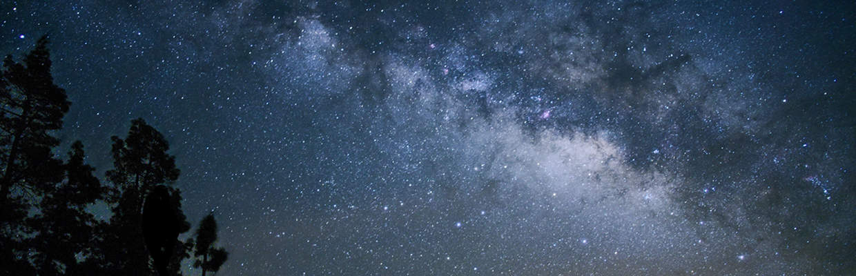
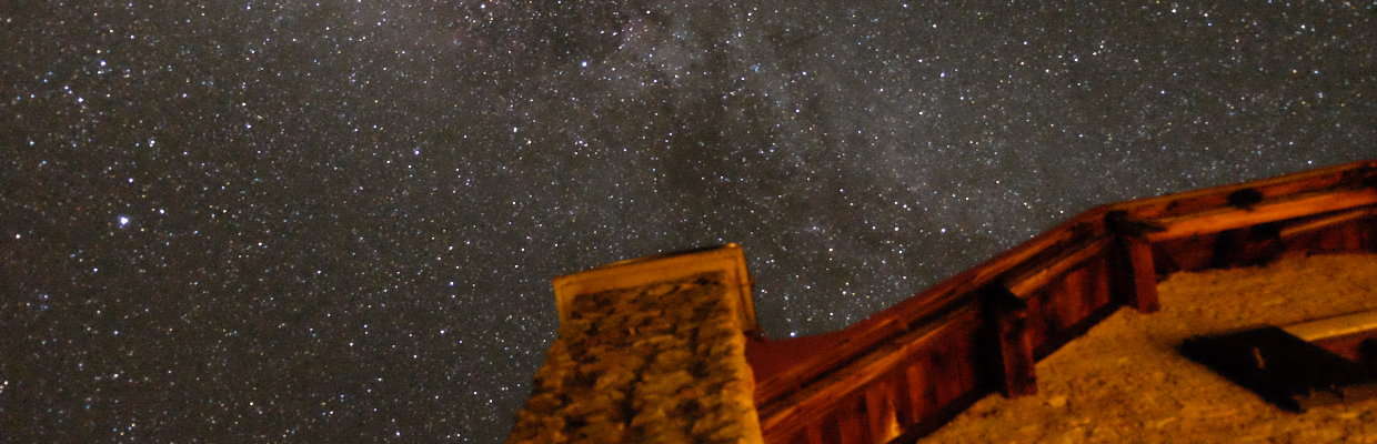
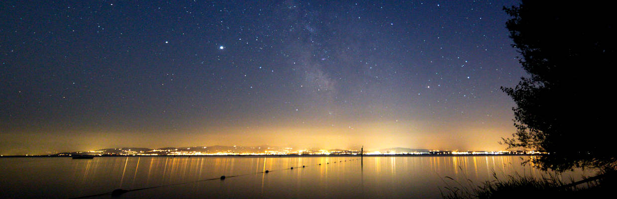
In this post I want to show a way of Milkyway image processing which does not require any commercial software product. The idea is to use rawtherapee, DeepSkyStacker and GIMP to develop, align and combine the frames to one final image.


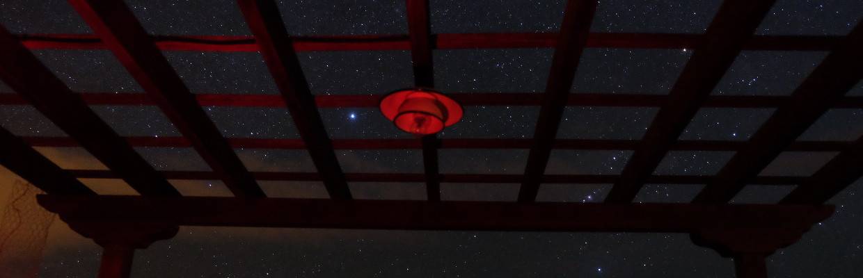
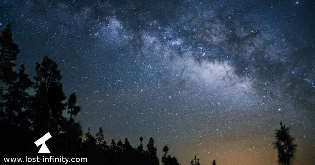
Camera: Fujifilm X-T1, Exposure time: 25sec. per frame, ISO: 1250, Aperture: f/2.8, focal length: 18mm

The problem

Quite often it is advantageous to use a high ISO value to get as much details as possible in the available exposure time (before the earth rotation becomes visible). On the other hand one probably does not want too much noise in the image. Therefore, the idea is to take multiple frames at a high ISO value and stack them later to reduce the noise. There is just one problem: The earth rotates and from frame to frame the stars are in different positions. Therefore an alignment of the frames before averaging is required. But then we get another problem: The foreground of each frame moves and so the resulting foreground gets fuzzy in the end. What to do?

Continue reading →

Night sky image processing – Part 7: Automatic Star Recognizer

In the parts 1-6 of my “Night sky image processing” Series I wrote about the different stages of night sky image processing. In this article I want to put all the pieces together and develop an “automatic star recognizer” which takes an astro-image as input and outputs a list of the recognized stars with their HFD and FWHM values.

The star recognizer processing pipeline

Basically the processing pipeline is as follows:

ROI = Region of interest

In order to achieve this I use most of the concepts I have looked into earlier:

As input I used this FITS image for testing.

Continue reading →

Night sky image processing – Part 6: Measuring the Half Flux Diameter (HFD) of a star – A Simple C++ implementation

In Part 5 of my “Night sky image processing” Series I wrote about measuring the FWHM value of a star using curve fitting. Another measure for the star focus is the Half Flux Diameter (HFD). It was invented by Larry Weber and Steve Brady. The main two arguments for using the HFD is robustness and less computational effort compared to the FWHM approach.

There is another article about the HFD available here. Another short definition of the HFD I found here. The original paper from Larry Weber and Steve Bradley is available here.

Definition of the HFD?

Let’s start with the definition: “The HFD is defined as the diameter of a circle that is centered on the unfocused star image in which half of the total star flux is inside the circle and half is outside.”

In a mathematical fashion this looks like this:

$$\sum\limits_{i=0}^{N} V_i \cdot (d_i – HFR) = 0 \Leftrightarrow HFR = \frac{\sum\limits_{i=0}^{N} V_i \cdot d_i}{\sum\limits_{i=0}^{N} V_i}$$

where:

  • $V_i$ is the pixel value minus the mean background value (!)
  • $d_i$ is the distance from the centroid to each pixel
  • $N$ is the number of pixels in the outer circle
  • $HFR$ is the Half Flux Radius for which the sum becomes $0$
Continue reading →

Night sky image processing – Part 4: Calculate the star centroid with sub-pixel accuracy

In Part 3 of my “Night sky image processing” Series I wrote about star-clustering. The result of this step was a list of stars and their pixels. The next step is to find the center of each star – the star centroid.

To keep it simple, in this example I apply the algorithm to calculate the star centroid only for one single star which I load from a FITS file. Mohammad Vali Arbabmir et. al.. proposed this algorithm in “Improving night sky star image processing algorithm for star sensors”.

Certainly it is possible to further optimize the implementation shown below. However, to me this is a good compromise between clarity and efficiency. The paper mentioned above will probably help a lot to get a better understanding of the implementation. Generally there are two steps:

Step 1: Calculation of the intensity weighted center (IWC) (to get an idea of where star center might be)

The calculation of IWC is based on the center of gravity CoG. The CoG is the same calculation as in physics but in this context just applied to an image. Each pixel brightness value has a weight – the brighter the “heavier”. For example to get the “center” x position $x_{cog}$ (this is the x position where the image has in x-direction the “brightest” value in mean. “In mean” means that all pixel values are considered). This directly leads to the following formulas for $x_{cog}$ and $y_{cog}$: 

$$x_{cog} = \frac{\sum_{x=0}^{N-1}\sum_{y=0}^{M-1} x \cdot I(x,y) }{\sum_{x=0}^{N-1}\sum_{y=0}^{M-1}I(x,y)}$$

$$y_{cog} = \frac{\sum_{x=0}^{N-1}\sum_{y=0}^{M-1} y \cdot I(x,y) }{\sum_{x=0}^{N-1}\sum_{y=0}^{M-1}I(x,y)}$$

The only thing that changes between the two formulas is $x$ and $y$. The denominator just normalized the expression so that a valid position comes out. In addition, $N$ is the image width, $Y$ is the image height and $I(x,y)$ is the pixel value at position $(x,y)$.

Now, the only difference in the calculation of IWC is that each pixel value is additionally weighted with it’s own value:  

Continue reading →

Night sky image processing – Part 3: Star clustering

Star clustering

This article is about finding all the pixels which belong to a star – also known as star clustering. A short C++ implementation based on CImg is shown below. In Part 2 of my “Night sky image processing” Series I was writing about thresholding. The result of the thresholding is a binary image. In this context it means the “1” pixels belong to stars, the “0” pixels belong to the background. I used Otsu’s method to calculate an according threshold value.

Introduction to star clustering

The binary image is now further examined in a process called clustering. In simple words the pixels which belong together (i.e. the neighbours) are grouped together. The result of this clustering process is a list of pixel groups which belong together – i.e. a list of stars and the pixels belonging to each star.

The implemented algorithm is based on the paper “Improving night sky star image processing algorithm for star sensors from Mohammad Vali Arbabmir et. al. However, in detail it is slightly different. My implementation assumes that the supplied image cannot be modified during the process. Hence I am using a set to put all white pixels into. To me this is a good compromise between memory consumption, performance and simplicity. However, the implementation can be further improved with respect to runtime performance when one would used a 2D array for the white pixels instead of a set.

The algorithm

The clustering algorithm is relatively straight forward:

Continue reading →