The Half Flux Diameter of a perfectly normal distributed star

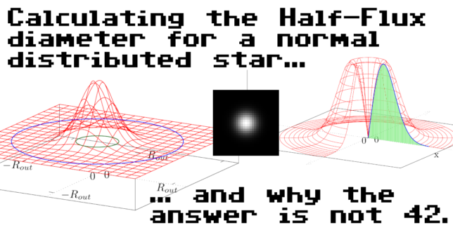
Calculating the Half Flux Diameter for a perfectly normal distributed star…

… and why the answer is not 42.

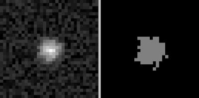
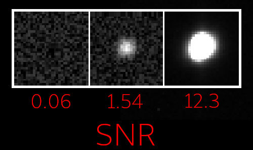
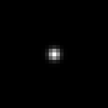
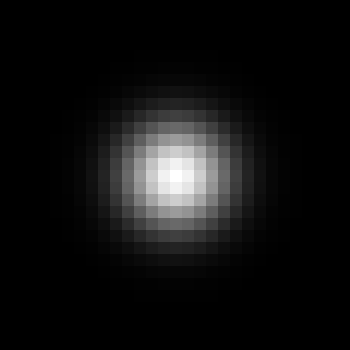
The goal of this article is to “manually” calculate the Half Flux Diameter (HFD) for a perfectly normal distributed star. Initially, I decided to add perfectly normal distributed stars with different σ values as additional unit tests to my focus finder software project. A few of those star images with σ=1, 2 and 3 are illustrated in figure 1.

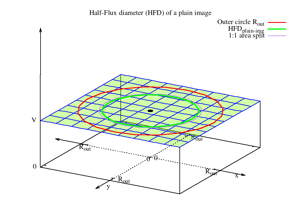
Previously, I examined the Half Flux diameter (HFD) for a plain image. In that article I cover some aspects in greater detail which I am reusing in this article. If something is unclear I recommend to read this article first.

σ=1
σ=2
σ=3

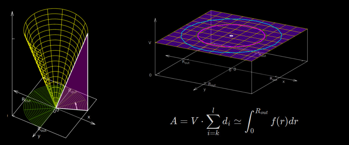
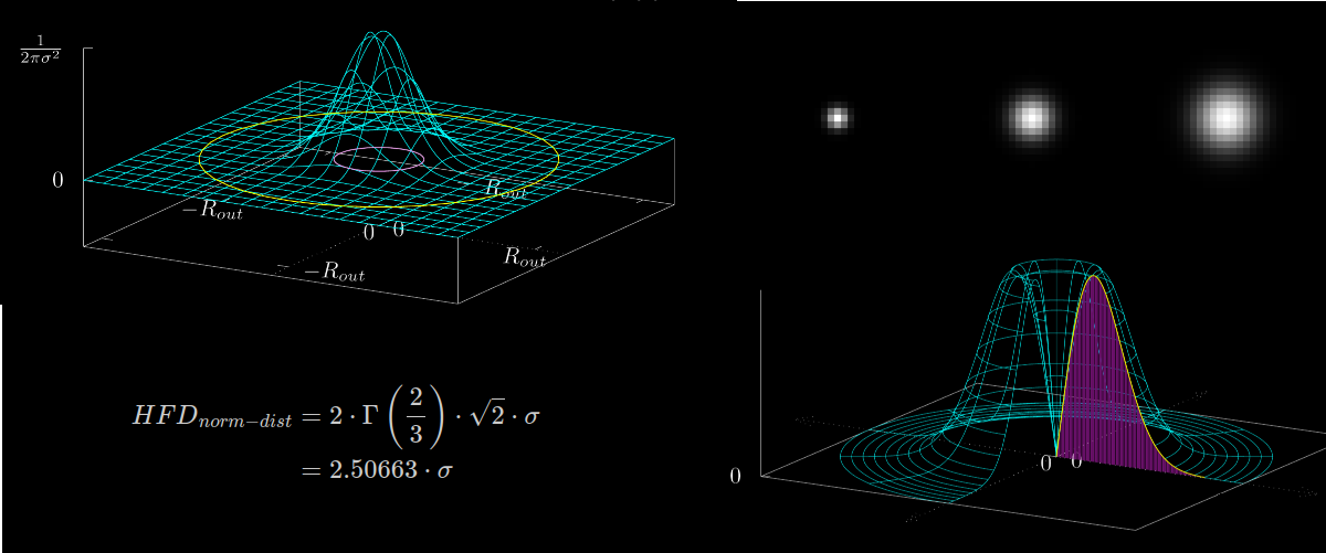
A 2D image can be represented in the 3D space where the $x$- and $y$-axis are used to express the position of the pixel and the $z$-axis to visualize the intensity (pixel value) – see figure 2 below.

Figure 2: The $x$- and $y$-axis represent the pixel position on the image plane, the $z$-axis represents the intensity $I$. The blue circle is the “outer circle” with radius $R_{out}$ up to which the pixel values are considered for the $HFD$ calculation. The green circle is the actual $HFD$ circle. The total volume under the surface is 1 (normalization factor is $\frac{1}{2\pi\sigma^2}$.

Following a similar approach like for the plain image, the Half Flux Diameter (HFD) for such an image will be derived in the following sections.

Quick summary

For those who just seek for the facts – here is a quick summary:

  • The Half Flux Diameter ($HFD$) for a perfectly normal distributed star is $HFD_{norm-dist} = 2 \cdot \Gamma\left(\frac{2}{3}\right) \cdot \sqrt{2} \cdot \sigma = 2.50663 \cdot \sigma$ where $\sigma$ is the variance of the distribution.
  • The result does not depend on $R_{out}$ and also not on the normalization factor of the distribution.
  • The expression was derived by converting the $HFD$ formula into an integral and inserting the normal distribution function as intensity (pixel value). The integral was solved by using a relation between the normal distribution and the $\Gamma$-function.
  • For the volume integration the second Pappus–Guldinus theorem is used.
Continue reading →

The Half Flux Diameter (HFD) of a plain image

Why the Half Flux Diameter (HFD) is not exactly what it suggests… and why it probably does not matter in practice.

For people dealing with astronomical images the Half Flux Diameter (HFD) definitely is a well known parameter. In a few words, the HFD measures how good (or not good) a star is in focus. The measure is relatively robust and also works when the star is far out of focus. In another article I cover the basics of the HFD.

Strange things happening here…

HFD and I were best friends until I started to write some unit tests for the HFD calculation routine in the focus finder project. Basically, the idea was to test the calculation routine with some test images for which the expected outcome was well known. This should have proven that the implemented routine was working correctly. One of those test images was a plain image in which all pixel values had the same value (> 0). Given the definition of the HFD:

“The HFD is defined as the diameter of a circle that is centered on the unfocused star image in which half of the total star flux is inside the circle and half is outside.”

it should be easy to predict the expected outcome. Since the flux is equally distributed across the entire image, it seems obvious that – as the name suggests – the resulting Half Flux Diameter is the diameter for which a corresponding “inner circle” contains exactly 50% of the area. The other 50% of the area should be located in between the “inner” – and the “outer” circle. This is what I assumed in my previous article about the HFD. However, it turned out to be wrong and I unfortunately have to invalidate this part.

Instead, the HFD routine gave a different result. Even for big images (to reduce the error of discretization) the result was off by a mysterious factor of 1,060660172 to the expected value. This gave reason to have a closer look to this enigma…

Quick Summary

For those who just seek for the facts – here is a quick summary

  • The Half Flux Diameter (HFD) of a plain image is $HFD_{plain-img} = \frac{4}{3} \cdot R_{out}$.
  • The corresponding HFD circle does not exactly split the area of the “outer circle” 1:1 even if the definition of the HFD suggests this – in other words $HFD_{plain-img}$ is not exactly $\sqrt{2} \cdot R_{out}$.
  • The root cause lies in the definition of the HFD itself: Pixels far away from the image center are weighted stronger than those which are very close.

For a few more details and reasoning read on…

Continue reading →

Fast “max entropy” thresholding for 16 bit images with CImg

In this article I shown a C++ implementation of the “max entropy” threshold algorithm using the CImg library. This implementation also performs for 16 and 32 bit / float images.

First, a little bit of context: Some time ago I implemented the OTSU threshold algorithm as a pre-processing step for image binarization. I used that threshold algorithm to distinguish the noise pixels from the potential “star” pixels. This worked quite well for the high contrast input images at that time. However, for weak stars it unfortunately failed badly.

Continue reading →

Easy 2D Signal-to-Noise Ratio (SNR) calculation for images to find stars without extracting the background noise (C++)

Calculation of a SNR for stars

This article shows how to calculate the 2D signal-to-noise ratio (SNR). Furthermore, it demonstrates how the $SNR$ can be used to decide if there is a potential star in the image.

Long story short – I was looking for a way to detect more or less reliably if a user selected a region which contains a star. I wanted to be able to clearly distinguish between the following two images:

Solution with the CImg library

After a long journey I finally ended up with the following solution. It is based on the CImg library which in a way calculates the Signal-to-noise ratio (SNR):

CImg <uint16_t> image;
...
double q = image.variance(0) / image.variance_noise(0);
double qClip = (q > 1 ? q : 1);
double snr = std::sqrt(qClip - 1);

For the two images above the code gives the following results:

~/snr$ ./snr no_star.fits 
SNR: 0.0622817
~snr$ ./snr test_star.fits
SNR: 1.5373

For many people this is where the journey ends. But for some of you it may just begin :). Follow me into the rabbit hole and find out why the solution shown above actually works…

Continue reading →

Finding perfect focus with V-Curve fitting based on a hyperbolic function

This article is about finding the best possible telescope focus by approximating a V-Curve with a hyperbolic function.

What is a V-Curve?

A V-Curve is the result of moving the focus of a telescope from an outside focus position into the focus and then further into the same direction out of focus again. This way a V-Curve comes into existence where the focus position is on the x-axis and the focus measure on the y-axis (right figure). Probably not surprising this curve is called V-Curve since it is similar to a V. There are different ways to measure the focus – for example the “Half-Flux Diameter” (HFD) and the “Full width at half maximum” (FWHM). In this case the I use the HFD measure.

Continue reading →