


This article is about finding the best possible telescope focus by approximating a V-Curve with a hyperbolic function.
What is a V-Curve?
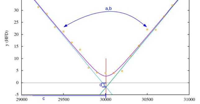
A V-Curve is the result of moving the focus of a telescope from an outside focus position into the focus and then further into the same direction out of focus again. This way a V-Curve comes into existence where the focus position is on the x-axis and the focus measure on the y-axis (right figure). Probably not surprising this curve is called V-Curve since it is similar to a V. There are different ways to measure the focus – for example the “Half-Flux Diameter” (HFD) and the “Full width at half maximum” (FWHM). In this case the I use the HFD measure.


From this V-Curve (or a set of those V-Curves) one wants to determine the ideal focus position. In order to do so, we need to extract more abstract criteria like slopes and / or local minimumfrom the individual data points. We can achieve this by approximating a function to the data points as good as possible and then take the respective curve parameters from the resulting function as such criteria. Executing the implementation below results in the figure shown on the top right.
Why using a hyperbolic curve?
What may be the advantages of a hyperbolic curve fitting?
- When fitting the data against two straight lines the algorithm must decide which data points go to which line. When fitting against one hyperbolic curve “as a whole”, this problem no longer exists.
- Because of the round shape at the bottom fitting two straight lines, is problematic since the program has to decide which data points close to the best focus position should still be part of the fitting and which should not. This problem no longer exists when using a hyperbolic curve.
Parameters of a hyperbolic curve
For a V-Curve as shown above there could be different ways to approximate it. They all have different advantages and disadvantages. For example one could try to use a parable or straight lines. In this approach I want to show the approximation to the V-Curve with a hyperbolic curve.
Consider the following explicit function: $$H(x,a,b,c,d) = b \cdot \sqrt{1 + \frac{\big(x-c\big)^2}{a^2}} + d$$
It describes a hyperbolic curve. $x$ is the variable and $a$, $b$, $c$ and $d$ are parameters which influence position and shape of the curve.
The following image illustrates an example of how this hyperbolic curve could look like for different parameter sets.


The figure above helps to understand the effect of the different function parameters: $a$ & $b$ define the “opening angle” of the hyperbolic curve, $c$ shifts the curve to the left or right on the x-axis and $d$ shifts the curve up- or down along the y-axis.
As one can see this is quite close to how a typical V-Curve of a telescope focusing run looks like. To the left and to the right the slope is constant and in the center it looks a little like a parable. Calculating the limiting values easily result in the left and the right tangent:
- Left: $\lim_{x\to-\infty}H(x,a,b,c,d) = -\frac{b}{\lvert a \rvert} \cdot \left(x-c\right) + d$
- Right: $\lim_{x\to\infty}H(x,a,b,c,d) = \frac{b}{\lvert a \rvert} \cdot \left(x-c\right) + d$
The picture above also shows the two tangents (green and turquoise).
NOTE: Since $H(x)$ is the same for $a$ and $-a$, for the equations of the tangents the absolute value of $a$ needs to be used. Otherwise, if $a$ is negative (like in the example), the left tangent would become the right tangent and vice versa. By using the absolute value $\lvert a \rvert$ this problem no longer exists. Many thanks to M. Velten from Astelco Systems for the hint.
Using the Levenberg-Marquart algorithm to approximate a hyperbolic curve to the V-Curve data points
The next step is to determine the parameters $a$, $b$, $c$ and $d$ of the hyperbolic curve for a given set of $(x,y)$ data points (in this context focuser position and HFD value). The goal is to calculate the parameters so that the resulting curve is as close to the data points as possible. The Levenberg-Marquart algorithm helps to achieve this. To avoid reinventing the wheel an implementation of this algorithm from the GNU Scientific Library (GSL) is used.
This algorithm requires the partial derivative of $H(x,a,b,c,d)$ to each parameter. The different partial derivatives make then up the Jacobi matrix $J$. Below is a list with the partial derivatives. To simplify the final expression we substitute a repeating expression with $\Phi(x)=\sqrt{\frac{(x-c)^2}{a^2} + 1}$. The code below also reflects $\Phi(x)$ with a function named phi().
$$\begin{align} \frac{\partial H}{\partial a} &= -b \cdot \frac{\left(x-c\right)^2}{a^3 \cdot \sqrt{1 + \frac{\left(x-c\right)^2}{a^2} }} = -\frac{b}{a^3} \cdot \frac{\left(x-c\right)^2}{\Phi(x)} \\ \frac{\partial H}{\partial b} &= \sqrt{1 + \frac{\left(x-c\right)^2}{a^2} } = \Phi(x) \\ \frac{\partial H}{\partial c} &= -\frac{b}{a^2} \cdot \frac{x-c}{\sqrt{1 + \frac{\left(x-c\right)^2}{a^2}}} = -\frac{b}{a^2} \cdot \frac{x-c}{\Phi(x)} \\ \frac{\partial H}{\partial d} &= 1 \\ \end{align}$$
This leads to the Jacobi matrix
$$\begin{align}
J &=
\begin{pmatrix}
\frac{\partial H}{\partial a} & \frac{\partial H}{\partial b} & \frac{\partial H}{\partial c} & \frac{\partial H}{\partial d}
\end{pmatrix} \\ &= \begin{pmatrix}
-\frac{b}{a^3} \cdot \frac{\left(x-c\right)^2}{\Phi(x)} & & & \Phi(x) & & & -\frac{b}{a^2} \cdot \frac{x-c}{\Phi(x)} & & & 1
\end{pmatrix}\end{align}$$
which will be used in the C++ program below to calculate an approximated hyperbolic curve.
In addition the Levenberg-Marquart algorithm requires the first and the second derivative of $H$ to $x$ :
$$H(x,a,b,c,d)^{\prime} = \frac{b \cdot (x-c)}{a^2 \cdot \sqrt{\frac{(x-c)^2}{a^2} + 1}} = \frac{b \cdot (x-c)}{a^2 \cdot \Phi(x)}$$
$$H(x,a,b,c,d)^{\prime\prime} = \frac{b}{a^2 \cdot \left(\frac{(x-c)^2}{a^2} + 1\right)^{\frac{3}{2}}} = \frac{b}{a^2 \cdot \Phi^3(x)}$$
Meaning of the V-Curve in an optical system
One important thing to note is that the shape of the V-Curve more or less characterizes the optical system consisting of focus, telescope and camera. This is independent of the current, absolute best focus position. That also means: Knowing the V-Curve of a system allows a quite good prediction of the best absolute focus position by just measuring a few data points. This can be helpful to quickly focus a system and move the more time consuming procedure of recording a whole V-Curve to the very beginning. Once such a V-Curve exists for a system, some algorithm can reuse it and save a lot of time during the focusing process.
C++ Implementation
With those thoughts we can now start to implement something:
#include <iostream>
#include <array>
#include <vector>
#include <list>
#include <algorithm>
#include <iostream>
#include <fstream>
#include <iterator>
#include <tuple> // For std::tie

#include <gsl/gsl_multifit_nlin.h>

using namespace std;

/**********************************************************************
 * Helper classes
 **********************************************************************/
struct DataPointT {
  float x;
  float y;
  DataPointT(float inX = 0, float inY = 0) : x(inX), y(inY) {}
};

typedef vector<DataPointT> DataPointsT;

struct GslMultiFitDataT {
  float y;
  float sigma;
  DataPointT pt;
};

typedef vector<GslMultiFitDataT> GslMultiFitParmsT;


/**********************************************************************
 * Curve to fit to is supplied by traits.
 **********************************************************************/
template <class FitTraitsT>
class CurveFitTmplT {
public:
  typedef typename FitTraitsT::CurveParamsT CurveParamsT;

  /**
   * DataAccessor allows specifying how x,y data is accessed.
   * See https://en.wikipedia.org/wiki/Approximation_error for expl. of rel and abs errors.
   */
  template<typename DataAccessorT> static int
  fitGslLevenbergMarquart(const typename DataAccessorT::TypeT & inData,
           typename CurveParamsT::TypeT * outResults, double inEpsAbs,
           double inEpsRel, size_t inNumMaxIter = 500) {
    GslMultiFitParmsT gslMultiFitParms(inData.size());

    // Fill in the parameters
    for (typename DataAccessorT::TypeT::const_iterator it = inData.begin(); it != inData.end(); ++it) {
      size_t idx = std::distance(inData.begin(), it);
      const DataPointT & dataPoint = DataAccessorT::getDataPoint(idx, it);
      gslMultiFitParms[idx].y     = dataPoint.y;
      gslMultiFitParms[idx].sigma = 0.1f;
      gslMultiFitParms[idx].pt    = dataPoint;
    }

    // Fill in function info
    gsl_multifit_function_fdf f;
    f.f      = FitTraitsT::gslFx;
    f.df     = FitTraitsT::gslDfx;
    f.fdf    = FitTraitsT::gslFdfx;
    f.n      = inData.size();
    f.p      = FitTraitsT::CurveParamsT::_Count;
    f.params = & gslMultiFitParms;


    // Allocate the guess vector
    gsl_vector * guess = gsl_vector_alloc(FitTraitsT::CurveParamsT::_Count);
    // Make initial guesses - here we just set all parameters to 1.0
    FitTraitsT::makeGuess(gslMultiFitParms, guess);
    // Create a Levenberg-Marquardt solver with n data points and m parameters
    gsl_multifit_fdfsolver * solver = gsl_multifit_fdfsolver_alloc(gsl_multifit_fdfsolver_lmsder,
                                         inData.size(), FitTraitsT::CurveParamsT::_Count);
    gsl_multifit_fdfsolver_set(solver, & f, guess);  // Initialize the solver

    int status, i = 0;

    // Iterate to to find a result
    do {
      i++;
      status = gsl_multifit_fdfsolver_iterate(solver); // returns 0 in case of success
      if (status) {  break; }
      status = gsl_multifit_test_delta(solver->dx, solver->x, inEpsAbs, inEpsRel);
    } while (status == GSL_CONTINUE && i < inNumMaxIter);

    // Store the results to be returned to the user (copy from gsl_vector to result structure)
    for (size_t i = 0; i < FitTraitsT::CurveParamsT::_Count; ++i) {
      typename FitTraitsT::CurveParamsT::TypeE idx =
                 static_cast<typename FitTraitsT::CurveParamsT::TypeE>(i);
      (*outResults)[idx] = gsl_vector_get(solver->x, idx);
    }

    // Free GSL memory
    gsl_multifit_fdfsolver_free(solver);
    gsl_vector_free(guess);

    return status;
  }
};


/**********************************************************************
 * Hyperbol fit traits
 **********************************************************************/
class HyperbolFitTraitsT {
private:

public:
  struct CurveParamsT {
    enum TypeE { A_IDX = 0, B_IDX, C_IDX, D_IDX, _Count };
    struct TypeT : public std::array<float, TypeE::_Count> {
      TypeT(const gsl_vector * inVec = 0) {
        for (size_t i = 0; i < TypeE::_Count; ++i) {
          TypeE idx = static_cast<TypeE>(i);
          (*this)[i] = (inVec ? gsl_vector_get(inVec, idx) : 0);
        }
      }
    };
  };

  /**
   * In this case we just initialize all parameters with 1.
   */
  static void makeGuess(const GslMultiFitParmsT & inData, gsl_vector * guess) {
    // Find min HFD -> good start value for c
    GslMultiFitParmsT::const_iterator minEl, maxEl;
    std::tie(minEl, maxEl) = std::minmax_element(begin(inData), end(inData),
                         [] (GslMultiFitDataT const& s1, GslMultiFitDataT const& s2)
                         {
                           return s1.pt.y < s2.pt.y;
                         });

    gsl_vector_set(guess, CurveParamsT::A_IDX, 1.0);
    gsl_vector_set(guess, CurveParamsT::B_IDX, 2.0);
    gsl_vector_set(guess, CurveParamsT::C_IDX, minEl->pt.x);
    gsl_vector_set(guess, CurveParamsT::D_IDX, 1.0);
  }

  /**
   * Phi() is a repeating part of the function calculation used by
   * different derivations.
   */
  static float phi(float x, float a, float c) {
    const float a2 = a * a;
    const float diff = x - c;
    const float diff2 = diff * diff;

    return sqrt(1.0 + (diff2 / a2));
  }

  /* H(x) */
  static float fx(float x, const CurveParamsT::TypeT & inParms) {
    const float a = inParms[CurveParamsT::A_IDX];
    const float b = inParms[CurveParamsT::B_IDX];
    const float c = inParms[CurveParamsT::C_IDX];
    const float d = inParms[CurveParamsT::D_IDX];

    return b * phi(x, a, c) + d;
  }

  /* Calculates H(x) for each data point. */
  static int gslFx(const gsl_vector * x, void * inGslParams, gsl_vector * outResultVec) {
    // Store the current coefficient values
    CurveParamsT::TypeT curveParams(x);

    // Store parameter values
    const GslMultiFitParmsT * gslParams = ((GslMultiFitParmsT*) inGslParams);
    // Execute Levenberg-Marquart on f(x)
    for(size_t i = 0; i < gslParams->size(); ++i) {
      const GslMultiFitDataT & gslData = gslParams->at(i);
      float yi = HyperbolFitTraitsT::fx((float) gslData.pt.x, curveParams);

      // TODO: Is this ok?
      gsl_vector_set(outResultVec, i, (yi - gslData.y) / gslData.sigma);
    }

    return GSL_SUCCESS;
  }

  /* Calculates the Jacobian (derivative) matrix  */
  static int gslDfx(const gsl_vector * x, void * params, gsl_matrix * J) {
    // Store parameter values
    const GslMultiFitParmsT * gslParams = ((GslMultiFitParmsT*) params);

    // Store current coefficients
    float a = gsl_vector_get(x, CurveParamsT::A_IDX);
    float b = gsl_vector_get(x, CurveParamsT::B_IDX);
    float c = gsl_vector_get(x, CurveParamsT::C_IDX);

    // Store non-changing calculations
    const float a2 = a * a;
    const float a3 = a * a2;

    for(size_t i = 0; i < gslParams->size(); ++i) {
      const GslMultiFitDataT & gslData = gslParams->at(i);

      const float oneBySigma = 1.0f / gslData.sigma;
      const float x = gslData.pt.x;
      const float x_minus_c = x - c;

      gsl_matrix_set(J, i, CurveParamsT::A_IDX,
           -oneBySigma * b * (x_minus_c * x_minus_c) / (a3 * phi(x, a, c)));
      gsl_matrix_set(J, i, CurveParamsT::B_IDX,
            oneBySigma * phi(x, a, c));
      gsl_matrix_set(J, i, CurveParamsT::C_IDX,
           -oneBySigma * b * x_minus_c / (a2 * phi(x, a, c)));
      gsl_matrix_set(J, i, CurveParamsT::D_IDX,
            oneBySigma);
    }

    return GSL_SUCCESS;
  }

  /* Invokes f(x) and f'(x) */
  static int gslFdfx(const gsl_vector * x, void * params, gsl_vector * f, gsl_matrix * J) {
    gslFx(x, params, f);
    gslDfx(x, params, J);

    return GSL_SUCCESS;
  }
};


/**********************************************************************
 * Calculation of asymptotes / slopes
 **********************************************************************/
float left_slope(float x, float a, float b, float c, float d) {
  return -(b/a) * (x-c) + d;
}
float right_slope(float x, float a, float b, float c, float d) {
  return (b/a) * (x-c) + d;
}


/**********************************************************************
 * Custom data structure + accessor
 **********************************************************************/
typedef pair<float, float> MyDataPointT;
typedef list<MyDataPointT> MyDataContainerT;

class MyDataAccessorT {
public:
  typedef MyDataContainerT TypeT;
  static DataPointT getDataPoint(size_t inIdx, TypeT::const_iterator inIt) {
    DataPointT dp(inIt->first /*inIdx*/, inIt->second /*y*/);
    return dp;
  }
};


/**********************************************************************
 * Main
 **********************************************************************/
int main(int argc,  char** argv) {

  // Check argument
  if (argc != 2) {
    std::cout << "Usage: hyperbol_fit <path/to/datafile>" << std::endl;
    return -1;
  }

  std::string filename(argv[1]);

  // Fill data container with some hyperbol shaped data
  MyDataContainerT dataPointsToFit;

  // Read data file
  std::ifstream infile(filename);
  MyDataPointT dp;
  while (infile >> dp.first >> dp.second) {
    dataPointsToFit.push_back(dp);
  }

  // Do the LM fit
  typedef CurveFitTmplT<HyperbolFitTraitsT> HyperbolMatcherT;
  typedef HyperbolMatcherT::CurveParamsT CurveParamsT;

  // Return value if fitGslLevenbergMarquart() is not evaluated here...
  CurveParamsT::TypeT hyperbolCurveParms;
  HyperbolMatcherT::fitGslLevenbergMarquart<MyDataAccessorT>(dataPointsToFit,
                        & hyperbolCurveParms, 0.1f /*EpsAbs*/, 0.1f /*EpsRel*/);

  // Print calculated curve parameters
  std::cout << "a=" << hyperbolCurveParms[CurveParamsT::A_IDX] << std::endl
        << "b=" << hyperbolCurveParms[CurveParamsT::B_IDX] << std::endl
        << "c=" << hyperbolCurveParms[CurveParamsT::C_IDX] << std::endl
        << "d=" << hyperbolCurveParms[CurveParamsT::D_IDX] << std::endl;

  return 0;
}
You can downoad the program here.
In order to compile it you need the following dynamic libraries:
- libgsl.so
- libgslcblas.so
- libboost_serialization.so
The following compile command should work if the required libraries are installed:
g++ -std=c++0x hyperbol_fit.cpp -lgsl -lgslcblas -lboost_serialization -o hyperbol_fit
Result
The following example V-Curve data (download) is used as input:
29000     40.5
29100     36.2
29200     31.4
29300     28.6
29400     23.1
29500     21.2
29600     16.6
29700     13.7
29800     6.21
29900     4.21
30000     3.98
30100     4.01
30200     4.85
30300     11.1
30400     15.3
30500     22.1
30600     21.9
30700     27.4
30800     32.1
30900     36.5
31000     39.7
Executing the program fits the hyperbolic curve to the V-Curve data:
$ ./hyperbol_fit vcurve.dat
a=-108.842
b=4.5666
c=30008.6
d=-1.85132
The result of the execution are the curve parameters $a$, $b$, $c$, and $d$. Those parameters have been entered into the following gnuplot script:
reset
a=-108.842
b=4.5666
c=30008.6
d=-1.85132
set term png size 1024,768 enhanced lw 2 font "Times,18"
set output "hyperbol_fit.png"
set contour
set cntrparam levels discrete 0
set view map
unset surface
set nokey
set isosamples 1000,1000
set autoscale x
set yrange [-5:42]
set xlabel "x (focus position)"
set ylabel "y (HFD)"
set title sprintf("H(x)=b*sqrt(1+(x-c)^2/a^2)+d, a=%i, b=%i, c=%i, d=%i", a, b, c, d)
set style line 1 lc rgb 'red' pt 5
H(x)=b*sqrt(1+(x-c)**2/a**2)+d
g(x)=-(b/a)*(x-c)+d
h(x)=+(b/a)*(x-c)+d
set arrow from c,-5 to c,10 nohead lc rgb 'red'
plot H(x),g(x),h(x),'vcurve.dat'
The script can be downloaded here. The overall result is shown below. As one can see the calculated hyperbolic curve fits the data points quite good. The red line indicates the theoretically optimal focus position which is expressed by parameter $c$.