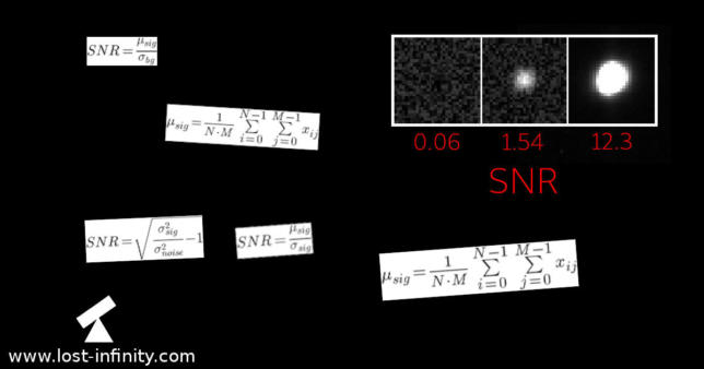
Calculation of a SNR for stars

This article shows how to calculate the 2D signal-to-noise ratio (SNR). Furthermore, it demonstrates how the $SNR$ can be used to decide if there is a potential star in the image.

Long story short – I was looking for a way to detect more or less reliably if a user selected a region which contains a star. I wanted to be able to clearly distinguish between the following two images:

Solution with the CImg library

After a long journey I finally ended up with the following solution. It is based on the CImg library which in a way calculates the Signal-to-noise ratio (SNR):

CImg <uint16_t> image;
...
double q = image.variance(0) / image.variance_noise(0);
double qClip = (q > 1 ? q : 1);
double snr = std::sqrt(qClip - 1);

For the two images above the code gives the following results:

~/snr$ ./snr no_star.fits 
SNR: 0.0622817
~snr$ ./snr test_star.fits
SNR: 1.5373

For many people this is where the journey ends. But for some of you it may just begin :). Follow me into the rabbit hole and find out why the solution shown above actually works…

SNR = SNR?

The initial definition of SNR

Before I decided to write this article, I knew the term $SNR$ basically from my studies in the field of electrical engineering. At that point in time it was basically a theoretical definition. The $SNR$ is somehow defined as the ratio of signal power to the noise power. This sounds logical but also is a bit abstract and may not help you much.

Basically when you look at that definition, you already see the problem: You need both, the “actual signal” and the “noise signal” in order to calculate the $SNR$. But more about that later….

The meaning of SNR in image processing

First, I would like to get further down to the actual meaning of the $SNR$ in image processing. For electrical signals measured in voltage it may be hard to exactly imagine what the definition above means. But for 2D signals – i.e. images – it is much easier to visualize the meaning of the signal-to-noise ratio $SNR$.

During my research I found some more or less valuable discussions about the calculation of the $SNR$. Some of then were on researchgate.net and on dspguide.com. But lets start with the definitions given by Wikipedia (at least for scientific purposes it is still a valuable source of information).

Traditionally, the $SNR$ has been defined as the ratio of the average signal value $\mu_{sig}$ to the standard deviation $\sigma_{bg}$ of the background:

$$SNR=\frac{\mu_{sig}}{\sigma_{bg}}$$

with

$$\mu_{sig}=\frac{1}{N \cdot M}\sum\limits_{i=0}^{N-1}\sum\limits_{j=0}^{M-1}x_{ij}$$

and

$$\sigma_{bg}=\sqrt{\frac{1}{N \cdot M} \sum\limits_{i=0}^{N-1}\sum\limits_{j=0}^{M-1} {\big(x_{ij} – \mu_{sig}\big)^2} }$$

So basically for the average signal $\mu_{sig}$ we sum up all pixel values and divide them by the number of pixels. This will result in an average “brightness” of the image. This goes to the numerator.

The denominator of the equation is the standard deviation of the background $\sigma_{bg}$. In other words it is the deviation from the mean pixel value for each single pixel. The standard deviation measures the strength of the noise. The higher the standard deviation, the stronger is the noise. This way the denominator increases with bigger noise and the $SNR$ decreases.

Getting rid of the chicken-and-egg problem

So far, so good. But as already mentioned above, we only have the one image. The image with the star which includes both – the signal (star) and the noise (background). Without additional effort (automatic detection or user interaction) a $SNR$ calculation program will not be able to calculate $\sigma_{bg}$.

In the first approach we try to get rid of this chicken-and-egg problem by applying an idea proposed in the same Wikipedia article (also when the intention behind is a different one):

In case of a “high-contrast” scene, many imaging systems set the background to uniform black. This forces $\sigma_{bg}$ to $0$. This way the previous definition of the $SNR$ does no longer work. Instead we replace $\sigma_{bg}$ by the standard deviation $\sigma_{sig}$ of the signal. This way we get a new definition for $SNR$:

$$SNR=\frac{\mu_{sig}}{\sigma_{sig}}$$

If you look at the equation you may notice that this $SNR$ only depends on the one image signal and no longer requires an extraction of the background signal.

So I thought this already is a possible solution. I implemented the following small program to test this algorithm on the given star image.

CImg<float> image;
.
.
.
double meanOfImage = image.mean();
double varianceOfImage = image.variance(0 /* 0 = second moment */);
double snr = meanOfImage / varianceOfImage;
  
std::cout << "SNR: " << snr << std::endl;

Executing this program gives the following result:

~/snr$ ./snr_high_contrast no_star.fits
SNR: 1.76239
~/snr$ ./snr_high_contrast test_star.fits
SNR: 0.604044
~/snr$ ./snr_high_contrast high_contrast_star.fits
SNR: 0.000659178

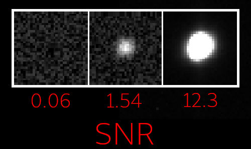
As you can see it is already possible to distinguish between having a star and not having a star. That’s actually good news. But the value somehow is inversely proportional and thus a little bit counter intuitive. At least from my perspective it would be nice if the SNR would increase if the signal increases compared to the noise. You could of course achieve that by inverting the fraction. But still one problem that remain is the great range in which the values can move. The following picture illustrates the different $SNR$ values for each star:

Yet another definition of SNR

Then I stumbled upon the following PDF document:

https://www2.ph.ed.ac.uk/~wjh/teaching/dia/documents/noise.pdf

It defines another $SNR$ as:

$$SNR=\sqrt{\frac{\sigma_{sig}^2}{\sigma_{noise}^2} – 1}$$

The document explains in detail how the $SNR$ can be calculated IF the noise can be measured somewhere in the image – e.g. in the background or at least the noise is known. Basically this is the same requirement as it was written in the Wikipedia article. However, this time I realized that it is sufficient to know how the noise looks like. This is of course equally true for the equation shown in the Wikipedia article. I did not put additional effort in researching this but I guess the noise in astronomical images is similar in most cases.

Based on this assumption we would be able to calculate a value for $\sigma_{bg}$ even if we have no image. Instead we estimate this value. When I looked closer to the CImg API I realized that this idea (of course…) is not new but there is even a function which is doing exactly that:

The CImg library provides a variance estimator function (variance_noise()):

https://cimg.eu/reference/structcimg__library_1_1CImg.html#a1c6097b1ed4f54e4b3ff331f6a2dc7d6

With this function a more or less typical noise is simulated. This way a more complicated background extraction and noise measurement does not need to be implemented. It is even possible to choose between different estimator functions. For my purpose I decided to use the “second moment” (variance_noise(0)) to calculate the noise estimation.

The final solution

This in the end lead to the final piece of code which turned out to work quite well:

#include <cmath> // std::sqrt()
#include <memory>
#include <iostream>
#include <CCfits/CCfits>
// Disable X11 dependency
#define cimg_display 0
#include <CImg.h>
using ImageT = cimg_library::CImg<uint16_t>;
void readFits(ImageT * outImg, const std::string & inFilename) {
  std::unique_ptr <CCfits::FITS> pInfile(new CCfits::FITS(inFilename, CCfits::Read, true));
  CCfits::PHDU& image = pInfile->pHDU();
  // read all user-specifed, coordinate, and checksum keys in the image
  image.readAllKeys();
  // Set image dimensions
  outImg->resize(image.axis(0) /*x*/, image.axis(1) /*y*/, 1 /*z*/, 1 /*1 color*/);
  // At this point the assumption that there is only 1 layer
  std::valarray<unsigned long> imgData;
  image.read(imgData);
  cimg_forXY(*outImg, x, y)
    {
      (*outImg)(x, outImg->height() - 1 - y) = imgData[outImg->offset(x, y)];
    }
}
int main(int argc, char *argv[]) {
  ImageT image;
  if (argc != 2) {
    std::cerr << "Usage: ./snr <my_fits_file.fits>" << std::endl; 
    return 1;
  }
  
  std::string filename = argv[1];
  
  try {
    readFits(& image, filename);
    double varianceOfImage = image.variance(0 /* 0 = Calc. variance as "second moment" */);
    double estimatedVarianceOfNoise = image.variance_noise(0 /* Uses "second moment" to compute noise variance */);
    double q = varianceOfImage / estimatedVarianceOfNoise;
    // The simulated variance of the noise will be different from the noise in the real image.
    // Therefore it can happen that q becomes < 1. If that happens it should be limited to 1.
    double qClip = (q > 1 ? q : 1);
    double snr = std::sqrt(qClip - 1);
  
    std::cout << "SNR: " << snr << std::endl;
    
  } catch(CCfits::FitsException & exc) {
    std::cerr << "Error loading FITS file: " << exc.message() << std::endl;
    return 1;
  }
  return 0;
}

The example above can be compiled like shown below. It requires three additional libraries. libCCfits and libcfitsio are just used for loading a FITS example file. I think the dependency to libpthread is introduced by libcfitsio.

~/snr$ g++ snr.cpp -lCCfits -lcfitsio -lpthread -o snr

The execution of the resulting program for the two different images above gives the following result:

~/snr$ ./snr no_star.fits 
SNR: 0.0622817
~/snr$ ./snr weak_star.fits 
SNR: 1.5373
~/snr$ ./snr high_contrast_star.fits
SNR: 12.2823

Conclusion and summary

When you look at those numbers they look somehow intuitive. For pure noise we have a small $SNR$ value. For a weak star the value is already about $25x$ times bigger and or a “high-contrast” star it is still significantly bigger. The following picture shows the different $SNR$ values for each star image:

The three test files can be downloaded here:

• https://www.lost-infinity.com/wp-content/uploads/no_star.fits
• https://www.lost-infinity.com/wp-content/uploads/weak_star.fits
• https://www.lost-infinity.com/wp-content/uploads/high_contrast_star.fits

In the end, when it turned out to be that easy, I was wondering if it is even worth to write an article about it. However, if you read upon here I hope it saved you some time 🙂 For further research I added the most important resources below:

• https://en.wikipedia.org/wiki/Signal-to-noise_ratio_(imaging)
• https://www.researchgate.net/post/How_is_SNR_calculated_in_images
• https://www.dspguide.com/ch25/3.htm
• https://www2.ph.ed.ac.uk/~wjh/teaching/dia/documents/noise.pdf
• https://nptel.ac.in/courses/117104069/chapter_1/1_11.html
• https://nptel.ac.in/courses/117104069/chapter_1/1_12.html
• https://kogs-www.informatik.uni-hamburg.de/~neumann/BV-WS-2010/Folien/BV-4-10.pdf

Clear skies!