Night sky image processing – Part 6: Measuring the Half Flux Diameter (HFD) of a star – A Simple C++ implementation

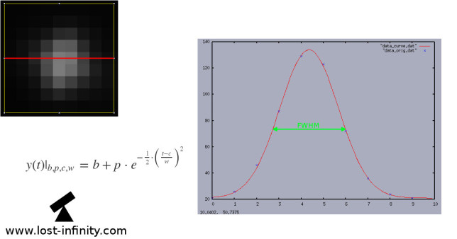
In Part 5 of my “Night sky image processing” Series I wrote about measuring the FWHM value of a star using curve fitting. Another measure for the star focus is the Half Flux Diameter (HFD). It was invented by Larry Weber and Steve Brady. The main two arguments for using the HFD is robustness and less computational effort compared to the FWHM approach.

There is another article about the HFD available here. Another short definition of the HFD I found here. The original paper from Larry Weber and Steve Bradley is available here.

Definition of the HFD?

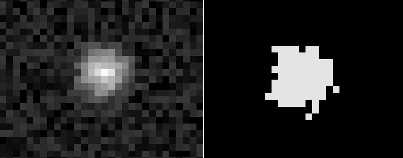
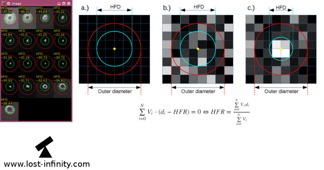
Let’s start with the definition: “The HFD is defined as the diameter of a circle that is centered on the unfocused star image in which half of the total star flux is inside the circle and half is outside.”

In a mathematical fashion this looks like this:

$$\sum\limits_{i=0}^{N} V_i \cdot (d_i – HFR) = 0 \Leftrightarrow HFR = \frac{\sum\limits_{i=0}^{N} V_i \cdot d_i}{\sum\limits_{i=0}^{N} V_i}$$

where:

  • $V_i$ is the pixel value minus the mean background value (!)
  • $d_i$ is the distance from the centroid to each pixel
  • $N$ is the number of pixels in the outer circle
  • $HFR$ is the Half Flux Radius for which the sum becomes $0$
Continue reading →

Night sky image processing – Part 5: Measuring FWHM of a star using curve fitting – A Simple C++ implementation

star_data

In Part 4 of my “Night sky image processing” Series I wrote about star centroid determination with sub-pixel accuracy. Based on this centroid position the FWHM determination of the star takes place. The FWHM (Full Width Half Maximum) value is a measurement for the star width. In this part I write about the so called curve-fitting which is helpful to determine the FWHM value from such an image. Note that for the following calculation and implementation I do not consider the sub-pixel determination of the centroid.

Determination of the FWHM

Let’s say we want to determine the FWHM in x-direction (red line). There is of course also one in y-direction. Basically, what happens is:

  1. Extract the pixel line through the centroid in x direction (those gray-level values usually form a Gaussian distribution: $$y(t)|_{b, p, c, w} = b + p \cdot e^{-\frac{1}{2} \cdot \big(\frac{t – c}{w}\big)^2}$$ We define a “data-point” as (x,y)=(pixel x-position, pixel gray-level value).
  2. Based on those (x,y) data-points determine the 4 parameters of a Gaussian curve so that the Gaussian curve and the data-points fit “as good as possible”. As fitting algorithm we use the so called “Levenberg-Marquart” algorithm. It tries to minimize the quadratic error between the data-points and the curve.
  3. The result is a Gaussian curve i.e. a parameter set which describes the curve (c=center, p=peak, b=base and the w=mean width). One of those parameters – the mean width is the FWHM value.
Continue reading →

Night sky image processing – Part 4: Calculate the star centroid with sub-pixel accuracy

In Part 3 of my “Night sky image processing” Series I wrote about star-clustering. The result of this step was a list of stars and their pixels. The next step is to find the center of each star – the star centroid.

To keep it simple, in this example I apply the algorithm to calculate the star centroid only for one single star which I load from a FITS file. Mohammad Vali Arbabmir et. al.. proposed this algorithm in “Improving night sky star image processing algorithm for star sensors”.

Certainly it is possible to further optimize the implementation shown below. However, to me this is a good compromise between clarity and efficiency. The paper mentioned above will probably help a lot to get a better understanding of the implementation. Generally there are two steps:

Step 1: Calculation of the intensity weighted center (IWC) (to get an idea of where star center might be)

The calculation of IWC is based on the center of gravity CoG. The CoG is the same calculation as in physics but in this context just applied to an image. Each pixel brightness value has a weight – the brighter the “heavier”. For example to get the “center” x position $x_{cog}$ (this is the x position where the image has in x-direction the “brightest” value in mean. “In mean” means that all pixel values are considered). This directly leads to the following formulas for $x_{cog}$ and $y_{cog}$: 

$$x_{cog} = \frac{\sum_{x=0}^{N-1}\sum_{y=0}^{M-1} x \cdot I(x,y) }{\sum_{x=0}^{N-1}\sum_{y=0}^{M-1}I(x,y)}$$

$$y_{cog} = \frac{\sum_{x=0}^{N-1}\sum_{y=0}^{M-1} y \cdot I(x,y) }{\sum_{x=0}^{N-1}\sum_{y=0}^{M-1}I(x,y)}$$

The only thing that changes between the two formulas is $x$ and $y$. The denominator just normalized the expression so that a valid position comes out. In addition, $N$ is the image width, $Y$ is the image height and $I(x,y)$ is the pixel value at position $(x,y)$.

Now, the only difference in the calculation of IWC is that each pixel value is additionally weighted with it’s own value:  

Continue reading →

Night sky image processing – Part 3: Star clustering

Star clustering

This article is about finding all the pixels which belong to a star – also known as star clustering. A short C++ implementation based on CImg is shown below. In Part 2 of my “Night sky image processing” Series I was writing about thresholding. The result of the thresholding is a binary image. In this context it means the “1” pixels belong to stars, the “0” pixels belong to the background. I used Otsu’s method to calculate an according threshold value.

Introduction to star clustering

The binary image is now further examined in a process called clustering. In simple words the pixels which belong together (i.e. the neighbours) are grouped together. The result of this clustering process is a list of pixel groups which belong together – i.e. a list of stars and the pixels belonging to each star.

The implemented algorithm is based on the paper “Improving night sky star image processing algorithm for star sensors from Mohammad Vali Arbabmir et. al. However, in detail it is slightly different. My implementation assumes that the supplied image cannot be modified during the process. Hence I am using a set to put all white pixels into. To me this is a good compromise between memory consumption, performance and simplicity. However, the implementation can be further improved with respect to runtime performance when one would used a 2D array for the white pixels instead of a set.

The algorithm

The clustering algorithm is relatively straight forward:

Continue reading →

Night sky image processing – Part 2: Image binarization using the Otsu thresholding algorithm

Otsu thresholding for star recognition

This article is about image binarization using the Otsu method. A simple C++ implementation of the Otsu thresholding algorithm based on the CImg library is shown. In Part 1 of my “Night sky image processing” series I have taken a look on anisotropic diffusion in order to reduce the image noise.

Introduction to Thresholding

The next topic I want to have a look at is thresholding. In this step the algorithm decides which pixels belong to the background and which pixels belong to a star. However, before the algorithm can decide which pixels belong to a particular star (also called clustering – see part 3) it first has to generally decide which pixels belongs to any star and which pixels belong to the background. This process is called thresholding i.e. converting a grey-scale image into a binary image. There are many different thresholding algorithms out there. All have there advantages and drawbacks. I found ImageJ very helpful to test different thresholding algorithms.

Why Otsu Thresholding for astro images

After trying different ones I found that Otsu’s method does a quite good job. After further reading I found out that this method is especially useful for images with bi-modal histograms. To my knowledge night shy images usually do not have bi-modal histograms. However, so far Otsu’s method still gave very good results with my star images. Furthermore it is relatively efficient and simple to implement. For those reasons I decided to go this way.

Introduction to Otsu Thresholding

Otsu’s algorithm tries to find the threshold so that the variance of all pixel values in the foreground and the variance of all pixel values in the background becomes minimal. The variance is a measure of the spread. The smaller the variance of for example the foreground pixel values, the closer the gray levels of the pixels and the more likely it is that they belong together. At least that’s how I understand Otsu’s method.

The following formula calculates a kind of “mean” variance $\sigma^2_{within}(th)$ of the foreground variance $\sigma^2_{fg}(th)$ and the background variance $\sigma^2_{bg}(th)$. In fact it is no mean but a weighted sum of both. The weights are the number of pixels in the respective group:

$$\sigma^2_{within}(th)=\sigma^2_{fg}(th) \sum\limits_{i=0}^{th-1} {num(i)} + \sigma^2_{bg}(th) \sum\limits_{i=th}^{N-1} {num(i)}$$

Continue reading →