
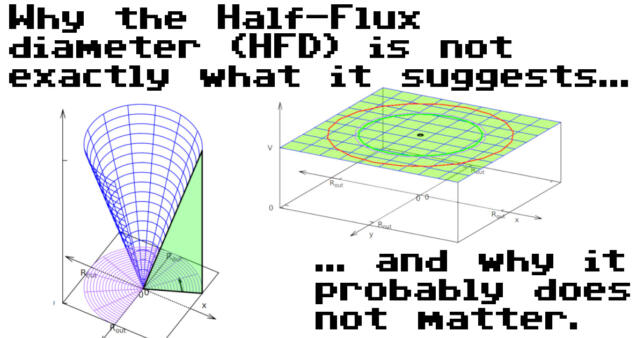
Why the Half Flux Diameter (HFD) is not exactly what it suggests… and why it probably does not matter in practice.
For people dealing with astronomical images the Half Flux Diameter (HFD) definitely is a well known parameter. In a few words, the HFD measures how well a star is focused. The measure is relatively robust and also works when the star is far out of focus. In another article I cover the basics of the HFD.
Strange things happening here…
HFD and I were best friends until I started to write some unit tests for the HFD calculation routine in the focus finder project. Basically, the idea was to test the calculation routine with some test images for which the expected outcome was well known. This should have proven that the implemented routine was working correctly. One of those test images was a plain image in which all pixel values had the same value (> 0). Given the definition of the HFD:
“The HFD is defined as the diameter of a circle that is centered on the unfocused star image in which half of the total star flux is inside the circle and half is outside.”
it should be easy to predict the expected outcome. Since the flux is equally distributed across the entire image, it seems obvious that – as the name suggests – the resulting Half Flux Diameter is the diameter for which a corresponding “inner circle” contains exactly 50% of the area. The other 50% of the area should be located in between the “inner” – and the “outer” circle. This is what I assumed in my previous article about the HFD. However, it turned out to be wrong and I unfortunately have to invalidate this part.
Instead, the HFD routine gave a different result. Even for big images (to reduce the error of discretization) the result was off by a mysterious factor of 1,060660172 to the expected value. This gave reason to have a closer look to this enigma…
Quick Summary
For those who just seek for the facts – here is a quick summary
- The Half Flux Diameter (HFD) of a plain image is $HFD_{plain-img} = \frac{4}{3} \cdot R_{out}$.
- The corresponding HFD circle does not exactly split the area of the “outer circle” 1:1 even if the definition of the HFD suggests this – in other words $HFD_{plain-img}$ is not exactly $\sqrt{2} \cdot R_{out}$.
- The root cause lies in the definition of the HFD itself: Pixels far away from the image center are weighted stronger than those which are very close.
For a few more details and reasoning read on…
Recap – Definition of the Half Flux Diameter (HFD)
There is already a more detailed article about the basics of the Half Flux Diameter (HFD) parameter on my blog. Still, here is a short recap about the aspects which are relevant in this context. Before defining the $HFD$ it is conceptually easier to first define the Half Flux Radius ($HFR$). The $HFR$ is implicitely defined as
$$\sum\limits_{i=0}^{N-1} V_i \cdot (d_i – HFR) = 0$$
In this equation $V_i$ is the pixel value of pixel $i$, $d_i$ denotes the distance of each pixel $i$ from the image center, $HFR$ represents the Half Flux Diameter and $N$ is the total number of pixels inside the “outer circle”.
All the “magic” in this first equation is, that the difference $d_i – HFR$ becomes negative for all the pixels inside the “inner circle” ($d_i < HFR$) and positive for all the pixels outside the “inner circle” ($d_i > HFR$). The $HFR$ therefore defines the circle for which the positive terms and the negative terms eliminate each other. The $HFR$ can be calculated by simply transposing this equation:
$$HFR = \frac{\sum\limits_{i=0}^{N-1} V_i \cdot d_i}{\sum\limits_{i=0}^{N-1} V_i}$$
The resulting Half Flux Diameter ($HFD$) is then defined as:
$$HFD = 2 \cdot HFR$$
Based on those definitions it is now possible to calculate the “theoretical” $HFD$ for a plain image.
Decomposing the HFD equation
A good starting point often is “divide and conquer”. Also in this case it turns out to be quite helpful. In a first step the formula of the $HFR$ will be decomposed into two parts. For this purpose two identifiers are being introduced – the nominator as “weighted distance sum” $WDS$ and the denominator as “pixel value sum” $PVS$. From now on the $HFR$ will be denoted as $HFR_{plain-img}$ since all is about the calculation of the $HFD$ of a plain image:
$$HFR_{plain-img} = \frac{WDS}{PVS} = \frac{\sum\limits_{i=0}^{N-1} V_i \cdot d_i}{\sum\limits_{i=0}^{N-1} V_i}$$
Part 1 – The “weighted distance sum” (WDS)
First, lets look at the upper part of the equation, the nominator:
$$WDS = \sum\limits_{i=0}^{N-1} V_i \cdot d_i$$
In case of a plain image, all pixels have the same value $V$ i.e. $V$ can be pulled in front of the sum:
$$WDS = V \cdot \sum\limits_{i=0}^{N-1} d_i$$
What remains is a sum of all the distances to all the pixels multiplied by $V$.
According to the definition of the $HFD$ above, the pixels denoted by $i=0..N-1$ are the ones which are located within the “outer circle”. The radius of this “outer circle” is denoted with $R_{out}$. All pixels outside that circle are not considered in the equation. This formula can be implemented straightforward in a computer program and if implemented correctly, the algorithm will give the correct $HFD$ value for a plain image.
However, in order to calculate the expected $HFD_{plain-img}$ “manually”, it is first helpful to transform the sum expression somehow into an integral. However, one needs to consider that even if there is just the one counter $i$, the operation takes place on an image – i.e. in two dimensions – and that there is the implicit condition that only pixels inside the “outer circle” should be considered.
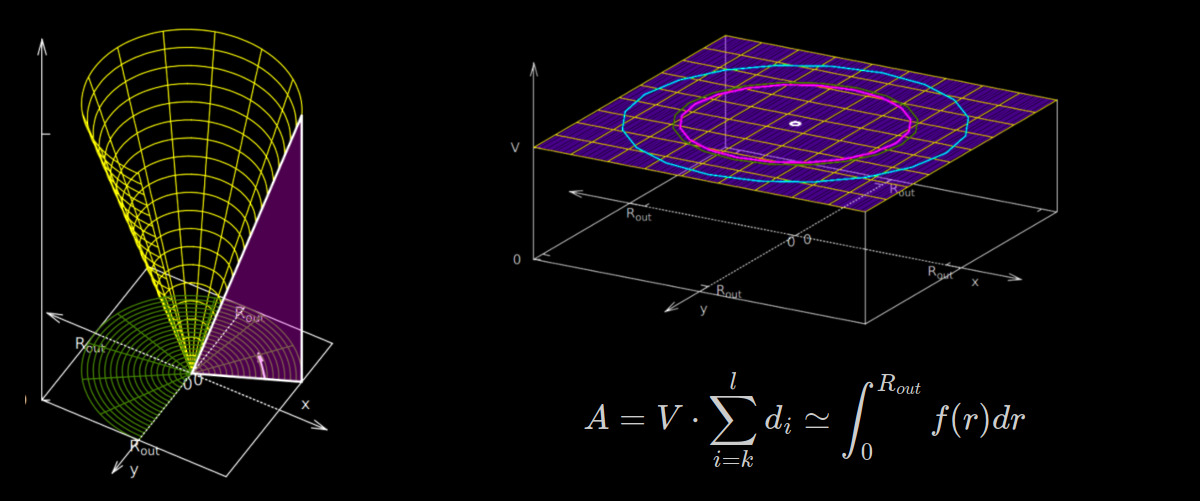
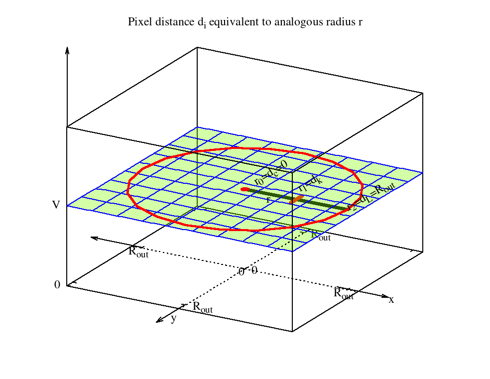
There are certainly multiple possibilities to calculate this and most likely more elegant ways than this one… However, there are many way to Rome… Looking at the $WDS$ equation again, one can see that $d_i$ measures the distance of each pixel to the image center. In other words, the center pixel of the image has the distance $r_0 = d_{c} = 0$, a pixel further away from the image center has the distance $r_1 = d_k$ and a pixel on the “outer circle” has the distance of $r_2 = d_L = R_{out}$ (see figure 1). That means the discretized distance $d_i$ can be modeled by an analogous radius $r$.
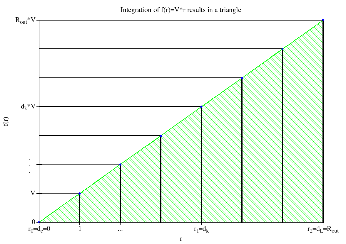
In $WDS$ all the $V_i \cdot d_i$ pairs are summed up in two dimensions. The same thing can be done similarly in the continuous space – for now in just one dimension – by integrating the function
$$f(r) = V \cdot r$$
from $0$ to $R_{out}$:
$$\begin{align}
A &= V \cdot \sum\limits_{i=k}^{l} d_i \simeq \int_{0}^{R_{out}} f(r) dr \\
&= V \cdot \int_{0}^{R_{out}} r dr \\
&= V \cdot \frac{R_{out}^2}{2}
\end{align}$$
$A$ is the area below the $f(r)$ function.The indices $k$ and $l$ denote the pixels along an arbitrary straight line from the image center to some point on the “outer circle”. As figure 2 illustrates, this is simply the area of a triangle.
The next step is to sum up all the infinite volume elements which are made up by $A$ and an infinitesimal angle $d\phi$ (see figure 3). This way all the $d_i \cdot V_i$ terms within the “outer circle” in the $xy$ image plane are included.
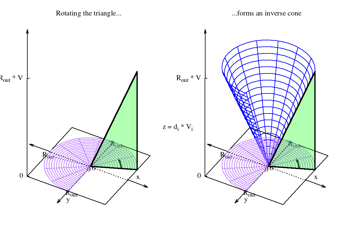
Geometrically the result can be interpreted as the volume of an “inverse” cone drawn-out by factor $V$. Since this shape can be easily composed by combining standard shapes, the corresponding volume formula can be easily derived without doing another integration step. In order to get the volume of the “inverse” cone, the volume of a corresponding cone needs to be subtracted from the volume of a corresponding cylinder (see figure 4).
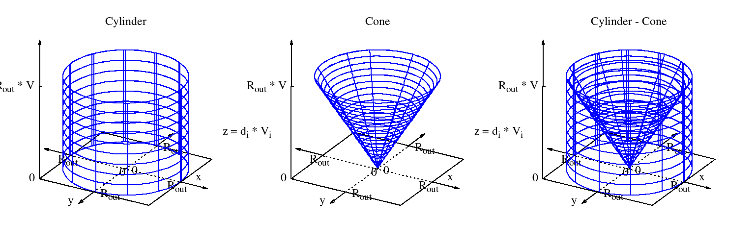
Give the following formulas of the volumes for a cylinder and a cone, the corresponding volume can be derived:
$$\begin{align}
V_{cylinder}&=A_{base} \cdot h \\
&= \pi \cdot r^2 \cdot h
\end{align}$$
With $h=R_{out} \cdot V$ the volume of the corresponding cylinder can be derived as
$$V_{cylinder} = \pi \cdot R_{out}^3 \cdot V$$
The volume of a corresponding cone can be derived in a similar way:
$$\begin{align}
V_{cone}&=\frac{1}{3} \cdot A_{base} \cdot h \\
&= \frac{1}{3} \cdot \pi \cdot r^2 \cdot h
\end{align}$$
Again, with $h=R_{out} \cdot V$ the volume of the corresponding cone is:
$$V_{cone} = \frac{1}{3} \cdot \pi \cdot R_{out}^3 \cdot V$$
Then the volume of the “inverse” cone is defined by:
$$\begin{align}
V_{cone-inv} &= V_{cylinder} – V_{cone} \\
&= V \cdot \pi \cdot R_{out}^3 – V \cdot \frac{1}{3} \cdot \pi \cdot R_{out}^3 \\
&= V \cdot \frac{2}{3} \cdot \pi \cdot R_{out}^3
\end{align}$$
Coming back to the beginning, this is the required expression for the weighted distance sum $WDS$:
$$\begin{align}
WDS &= V_{cone-inv} \\
&= V \cdot \frac{2}{3}\cdot \pi \cdot R_{out}^3
\end{align}$$
Part 2 – The “pixel value sum” (PVS)
For the second term in the $HFR_{plain-img}$ equation, the “pixel value sum” $PVS$ it is relatively easy to see how the analogous variant should look like. Since all $V_i=V$, the $V$ again can be moved in front of the sum:
$$PVS={V \cdot \sum\limits_{i=0}^{N-1}1}$$
What remains is in fact just $V$ times the sum of pixels in the “outer circle”. This is nothing else than the area of the “outer circle”. With this assumption, the $PVS$ turns into:
$$PVS = V \cdot \pi \cdot R_{out}^2$$
Putting everything back together
Now both parts of the $HFR$ equation have been transformed into expressions in the analogous space:
$$WDS = V \cdot \frac{2}{3}\cdot \pi \cdot R_{out}^3$$
$$PVS = V \cdot \pi \cdot R_{out}^2$$
Putting them back together finally results in a formula to calculate $HFR_{plain-img}$:
$$\begin{align}
HFR_{plain-img} &= \frac{WDS}{PVS} \\
&= \frac{V \cdot \frac{2}{3}\cdot \pi \cdot R_{out}^3}{V \cdot \pi \cdot R_{out}^2} \\
&= \frac{2}{3} \cdot R_{out}
\end{align}$$
As one can see the $V$ does not matter for the resulting $HFR_{plain-img}$ – what is actually expected. The resulting $HFR_{plain-img}$ for a completely grey and a completely white image should be the same.
With this result the expected $HFD_{plain-img}$ for a completely plain image (pixel values > 0) can be finally derived:
$$\begin{align}
HFD_{plain-img} &=2 \cdot HFR_{plain-img} \\
&= \frac{4}{3} \cdot R_{out}
\end{align}$$
Conclusion
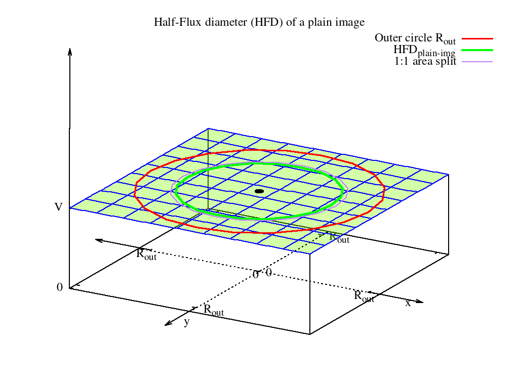
The Half Flux Diameter (HFD) of a plain image was “manually” calculated and comes down to $HFD_{plain-img} = \frac{4}{3} \cdot R_{out}$. That means that the corresponding $HFD$ circle is not exactly splitting the area of the “outer circle” 1:1 even if the definition of the $HFD$ suggests this.
This now also explains why the result of the $HFD$ computed by the machine was off by a mysterious factor of 1,060660172 compared to the diameter for which the two areas were exactly divided 1:1. The diameter of such a circle would be $\sqrt{2} \cdot R_{out}$ (see here for a derivation). This value was expected n the unit test. With the correct expectation value $\frac{4}{3} \cdot R_{out}$, the factor of 1,060660172 can be easily computed as $\frac{\sqrt{2}}{\frac{4}{3}}$.
Figure 5 illustrates $HFD_{plain-img}$ (green) in comparison to the circle which halves the area 1:1 (purple).

As one can see this diameter is slightly smaller than the purple one. Between the two diameters lies the factor 1,060660172.
So why doesn’t the $HFD$ of a pain image split the area 1:1 as the definition suggests? The root cause lies in the definition of the HFD itself: Pixels far away from the image center are weighted stronger than those which are very close.
When using the $HFD$ as a focus measure in practice, this factor most likely does not have any impact. However, in certain corner cases – like this one – it is helpful to know that the Half Flux Diameter (HFD) is not exactly what it suggests.
Clear skies!
Thanks for the theoretical explanation. A few years ago I found and offset of 6.4% by simulation of a Gaussian star shape of hundreds of pixel wide but could not explain it. That 6.4% value I did put in Wikipedia.