Night sky image processing – Part 7: Automatic Star Recognizer

In the parts 1-6 of my “Night sky image processing” Series I wrote about the different stages of night sky image processing. In this article I want to put all the pieces together and develop an “automatic star recognizer” which takes an astro-image as input and outputs a list of the recognized stars with their HFD and FWHM values.

The star recognizer processing pipeline

Basically the processing pipeline is as follows:

ROI = Region of interest

In order to achieve this I use most of the concepts I have looked into earlier:

As input I used this FITS image for testing.

Continue reading →

Night sky image processing – Part 6: Measuring the Half Flux Diameter (HFD) of a star – A Simple C++ implementation

In Part 5 of my “Night sky image processing” Series I wrote about measuring the FWHM value of a star using curve fitting. Another measure for the star focus is the Half Flux Diameter (HFD). It was invented by Larry Weber and Steve Brady. The main two arguments for using the HFD is robustness and less computational effort compared to the FWHM approach.

There is another article about the HFD available here. Another short definition of the HFD I found here. The original paper from Larry Weber and Steve Bradley is available here.

Definition of the HFD?

Let’s start with the definition: “The HFD is defined as the diameter of a circle that is centered on the unfocused star image in which half of the total star flux is inside the circle and half is outside.”

In a mathematical fashion this looks like this:

$$\sum\limits_{i=0}^{N} V_i \cdot (d_i – HFR) = 0 \Leftrightarrow HFR = \frac{\sum\limits_{i=0}^{N} V_i \cdot d_i}{\sum\limits_{i=0}^{N} V_i}$$

where:

  • $V_i$ is the pixel value minus the mean background value (!)
  • $d_i$ is the distance from the centroid to each pixel
  • $N$ is the number of pixels in the outer circle
  • $HFR$ is the Half Flux Radius for which the sum becomes $0$
Continue reading →

Night sky image processing – Part 5: Measuring FWHM of a star using curve fitting – A Simple C++ implementation

star_data

In Part 4 of my “Night sky image processing” Series I wrote about star centroid determination with sub-pixel accuracy. Based on this centroid position the FWHM determination of the star takes place. The FWHM (Full Width Half Maximum) value is a measurement for the star width. In this part I write about the so called curve-fitting which is helpful to determine the FWHM value from such an image. Note that for the following calculation and implementation I do not consider the sub-pixel determination of the centroid.

Determination of the FWHM

Let’s say we want to determine the FWHM in x-direction (red line). There is of course also one in y-direction. Basically, what happens is:

  1. Extract the pixel line through the centroid in x direction (those gray-level values usually form a Gaussian distribution: $$y(t)|_{b, p, c, w} = b + p \cdot e^{-\frac{1}{2} \cdot \big(\frac{t – c}{w}\big)^2}$$ We define a “data-point” as (x,y)=(pixel x-position, pixel gray-level value).
  2. Based on those (x,y) data-points determine the 4 parameters of a Gaussian curve so that the Gaussian curve and the data-points fit “as good as possible”. As fitting algorithm we use the so called “Levenberg-Marquart” algorithm. It tries to minimize the quadratic error between the data-points and the curve.
  3. The result is a Gaussian curve i.e. a parameter set which describes the curve (c=center, p=peak, b=base and the w=mean width). One of those parameters – the mean width is the FWHM value.
Continue reading →

Night sky image processing – Part 4: Calculate the star centroid with sub-pixel accuracy

In Part 3 of my “Night sky image processing” Series I wrote about star-clustering. The result of this step was a list of stars and their pixels. The next step is to find the center of each star – the star centroid.

To keep it simple, in this example I apply the algorithm to calculate the star centroid only for one single star which I load from a FITS file. Mohammad Vali Arbabmir et. al.. proposed this algorithm in “Improving night sky star image processing algorithm for star sensors”.

Certainly it is possible to further optimize the implementation shown below. However, to me this is a good compromise between clarity and efficiency. The paper mentioned above will probably help a lot to get a better understanding of the implementation. Generally there are two steps:

Step 1: Calculation of the intensity weighted center (IWC) (to get an idea of where star center might be)

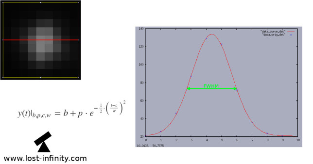
The calculation of IWC is based on the center of gravity CoG. The CoG is the same calculation as in physics but in this context just applied to an image. Each pixel brightness value has a weight – the brighter the “heavier”. For example to get the “center” x position $x_{cog}$ (this is the x position where the image has in x-direction the “brightest” value in mean. “In mean” means that all pixel values are considered). This directly leads to the following formulas for $x_{cog}$ and $y_{cog}$: 

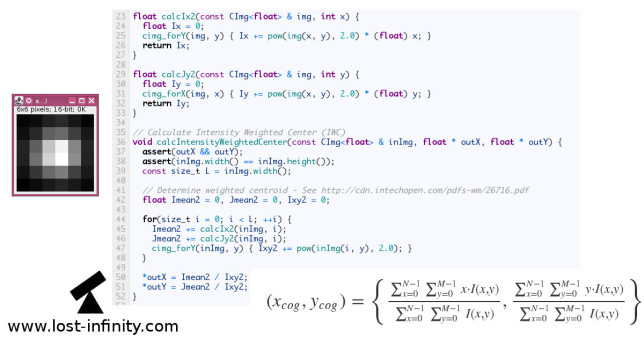
$$x_{cog} = \frac{\sum_{x=0}^{N-1}\sum_{y=0}^{M-1} x \cdot I(x,y) }{\sum_{x=0}^{N-1}\sum_{y=0}^{M-1}I(x,y)}$$

$$y_{cog} = \frac{\sum_{x=0}^{N-1}\sum_{y=0}^{M-1} y \cdot I(x,y) }{\sum_{x=0}^{N-1}\sum_{y=0}^{M-1}I(x,y)}$$

The only thing that changes between the two formulas is $x$ and $y$. The denominator just normalized the expression so that a valid position comes out. In addition, $N$ is the image width, $Y$ is the image height and $I(x,y)$ is the pixel value at position $(x,y)$.

Now, the only difference in the calculation of IWC is that each pixel value is additionally weighted with it’s own value:  

Continue reading →